SUBTOTAL
Using the SUBTOTAL Function in Excel
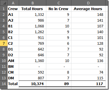
Tue, 06/10/2015 - 9:43am — jethroThe Subtotal function is commonly used when creating Subtotals on a table with the Data | Subtotals Menu command. However it can be just as easily used by writing the formula and has some powerful uses.
The syntax is SUBTOTAL(function_num,ref1,ref2,...)
The function numbers allow you to use any of the following functions in the subtotal:
|
Function_num |
Function_num |
Function |
|
1 |
101 |
AVERAGE |
|
2 |
102 |
COUNT |
|
3 |
103 |
COUNTA |
|
4 |
104 |
MAX |
|
5 |
105 |
MIN |
|
6 |
106 |
PRODUCT |
|
7 |
107 |
STDEV |
|
8 |
108 |
STDEVP |
|
9 |
109 |
SUM |
|
10 |
110 |
VAR |
|
11 |
111 |
VARP |
The most common is of course the SUM function.
When and why should you use SUBTOTAL and not just the SUM function on its own.
The SUBTOTAL function has some powerful abilities that the commonly used SUM function doesn't. For example when summing a list of cells that contains hidden rows or columns the SUM function will include them. However the SUBTOTAL function only operates on visible cells. The values of the hidden cells are excluded from the total. This is especially useful when filtering a list if you want to see the total of the visible (or filtered) cells.
Note by default, if you have a filtered list of values and you double click the sum (sigma) icon on the toolbar after you select a cell below the bottom of the filtered range Excel will not use a SUM formula but automatically use a SUBTOTAL function.
The SUBTOTAL function ignores other subtotals within the range. So if you have several subtotals and a grand total, the grand total formula can be the subtotal of the entire range that includes the subtotals and it will ignore them.
Links to my other Articles about Subtotals including using outlining.
http://www.spyjournal.biz/exceltips/2005/03/creating-subtotals-in-excel.html
http://www.spyjournal.biz/data_filters_in_Excel_2003_and_2007
Introduction to the new tables in Excel 2010
Fri, 27/04/2012 - 10:36am — jethroAs the title says this just an introduction. Its aimed at non power users who have recently moved to Office 2010 or 2007 from Excel 2003.
The main reason for this article is to demonstrate the basic use of the new table features and the ribbon features available to users.
I am going to start with showing you how to make a table from existing data and demonstrate a few of the ribbon features. I wont be going into anything too complicated in this post. Depending on feedback I might write some more specific detailed feature articles on table components and using tables later including converting tables back to ranges..
So how do we make a table – its actually very simple. In the following screenshots you will see a fairly typical spreadsheet with some information in it. I will show you how to turn that into a table.
Select any cell in the table.
From the Home Tab on the Ribbon click on the Format as Table Button.
Back To Basics: Data Filters in Excel 2003 and Excel 2007
Thu, 19/06/2008 - 2:38am — jethroData Filters are a very powerful way of analysing tables of data in Excel. Put simply they are a way of reducing the table down to just the items you want to see based on the selections you choose.
For example a simple table like this one, may have several hundred or thousand rows of data. However there may be only a few lines you are interested in. For example you may be only interested in people under the age of 18 or sales amounts that are negative (indicating a refund) or only see sales of red Ferraris.
Turning on the Filters
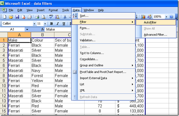
In Office 2003 Turn on the filters by selecting any cell in your table (contiguous section of data) and selecting Data, Filter, Auto Filter from the menu. (Keystroke ALT D F F)
The arrows will show up as in the next picture.


Recent comments
10 years 38 weeks ago
10 years 38 weeks ago
10 years 39 weeks ago
10 years 39 weeks ago
10 years 39 weeks ago
10 years 39 weeks ago
10 years 39 weeks ago
10 years 39 weeks ago
10 years 39 weeks ago
10 years 39 weeks ago