Introduction to the new tables in Excel 2010
As the title says this just an introduction. Its aimed at non power users who have recently moved to Office 2010 or 2007 from Excel 2003.
The main reason for this article is to demonstrate the basic use of the new table features and the ribbon features available to users.
I am going to start with showing you how to make a table from existing data and demonstrate a few of the ribbon features. I wont be going into anything too complicated in this post. Depending on feedback I might write some more specific detailed feature articles on table components and using tables later including converting tables back to ranges..
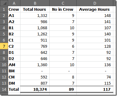
So how do we make a table – its actually very simple. In the following screenshots you will see a fairly typical spreadsheet with some information in it. I will show you how to turn that into a table.
Select any cell in the table.
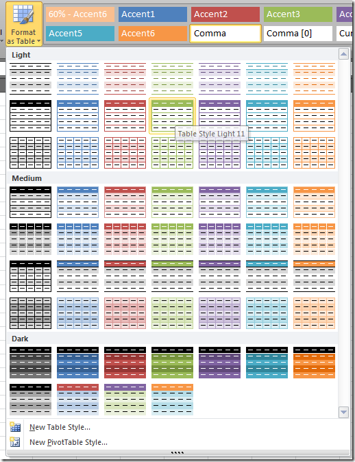
From the Home Tab on the Ribbon click on the Format as Table Button.
Select an option – don't worry too much about which one at this point – you can change it later if you need to.
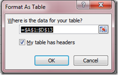
A dialog box asking where your table data is located will appear.
In this case it has found my data correctly. This is not a named range at this point but it will dynamically alter later as you add more rows or columns so you don’t need to make it any longer at the moment. If you already have headers then the tick box for “My table has headers” should be ticked. Click OK.
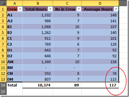
Notice that the table range is now highlighted and that it has ignored the pre-existing total line. In fact this should now be deleted as the table functions include totals that work better in most cases. I have circled the bottom right corner. This grab handle is available for resizing the table to include more rows or columns. I wont demonstrate that this time but feel free to have a play with it.
Now selecting any cell in the new table will expose on the ribbon a contextual tab called Table Tools | Design that was not previously available. These tools are only available to work with a table so unless you actually select a table the ribbon does not show this tab. The style options out to the right allow you to change the look of the table to suit your visual needs. Note these are theme related so as you change the spreadsheet theme these will also change.
I’m going to show you how to add a new total row. It’s pretty simple. Click the Total row Check box.
Feel free to play with the other options here also. However I want to demonstrate this one particularly because all the other options only affect the style or view except the header row which gives you access to filters. The total row gives you a whole new set of options by utilising the SUBTOTAL function. (More on this in an old post: Back To Basics: Data Filters in Excel 2003 and Excel 2007)
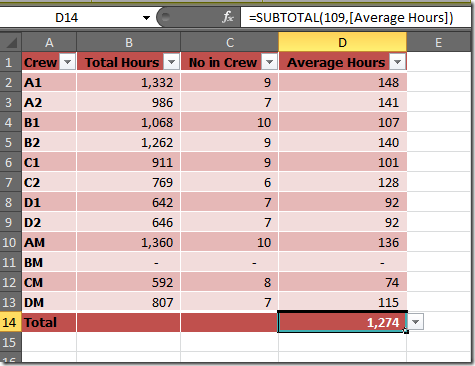
By default turning on the total row gives you only a single total in the furthest right hand column.
Click on this new cell and lets have a look at the formula.
Notice the syntax. =SUBTOTAL(109,[Average Hours]) I wont go into the whole SUBTOTAL function here – that will be the topic of another post in the future. However the 109 code here means SUM and the [Average Hours] is a table defined range name based on the header cell to refer to the data in cells D2:13. Note this is a dynamic range meaning if you add a 14th data row or delete a row the subtotal will still work on all the data cells in this column.
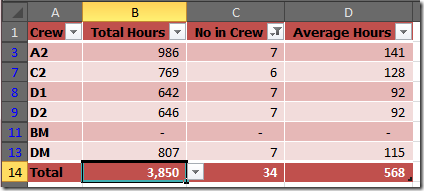
One other point to note about the SUBTOTAL formula – it works on visible cells only. This means that if you use the filters in the header row to change what is visible the subtotal value will reflect the sum of only the visible cells. Of course you can change this if necessary by using a different function – eg SUM or AVERAGE.
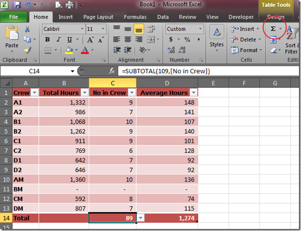
Finally we need to put subtotals into columns B and C. unfortunately copying the formula from Column D doesn’t work, as it will still refer to the [Average Hours] range. You could copy the formula and then edit each one so that the name in the [square brackets] is the same as the header for the column.
There is an easy way however.
Select the empty cell in the total line for Column C. Click the Home tab on the Ribbon and then click the Sigma (SUM) sign.
This will give you a SUBTOTAL total for Column C. Repeat for column B and you have a dynamically updating table with subtotals that change based on the filters.
See this view of the table filtered for all crews with less than 8 in the crew.
As usual comments and questions are welcomed.







Recent comments
10 years 38 weeks ago
10 years 38 weeks ago
10 years 39 weeks ago
10 years 39 weeks ago
10 years 39 weeks ago
10 years 39 weeks ago
10 years 39 weeks ago
10 years 39 weeks ago
10 years 39 weeks ago
10 years 39 weeks ago