IF
How to remove #N/A errors in Excel
Fri, 14/12/2012 - 12:21pm — jethroToday I had an email request:
I wasn't sure how to post, or join so I'm sending my question to you this way. I cannot figure out how to remove the #N/A error in LOOKUP. If the cells are blank it returns the #N/A error - I'd like to return either a blank or 0 instead. How do I do that? Her is my formula. (I'm sure you can tell by my formula I'm a rookie at this.) Any help is appreciated. Thanks!
=SUM((LOOKUP(B6,{1,2,3,4,5},{40,30,20,10,0}))+(LOOKUP(C6,{1,2,3,4,5},{40,30,20,10,0})+(LOOKUP(D6,{1,2,3,4,5},{40,30,20,10,0})+(LOOKUP(E6,{1,2,3,4,5},{40,30,20,10,0})+(LOOKUP(F6,{1,2,3,4,5},{40,30,20,10,0}))))))
 I have written a post on this before when I explained the ISNA function.
In this case I will break down the first component of the formula and show you how to insert it.
First of all understand that because this formula is summing components that are lookups, if any one of them returns an error than the overall sum will be an error even if the rest is not an error.
So to fix =LOOKUP(B6,{1,2,3,4,5},{40,30,20,10,0}) when it displays #N/A (eg if B6 is less than 1) we would use this function:
=IF(ISNA(LOOKUP(B6,{1,2,3,4,5},{40,30,20,10,0}))=TRUE,0,LOOKUP(B6,{1,2,3,4,5},{40,30,20,10,0}))
The same concept could be used for each lookup component. In this case the formula would become very involved so there might be easier ways to do it. Sometimes breaking the individual components our into individual cells and then summing them is a way to give more visible results – and easily see which component is causing the error.
So Lois – i hope that helps – and thanks for liking us on Facebook!
A practical way to use the IF function in Excel
Fri, 25/05/2012 - 11:09am — jethroThe IF function is a very useful logical tool. I have written an explanation on the IF Function before so I wont repeat that here. There are a number of other posts also that incorporate the use of the IF Function.
 What I want to do is highlight a useful way to use the IF function.
I use it a lot to compare lists of data. today I had been sent some data in a spread sheet that contained email addresses. I had to create a mail out to those email addresses and when i did that I received a number of bounce backs for incorrect email addresses. I then received a second email from the original person containing a revised spread sheet with the corrections to email addresses. given that there were a large number of addresses and only a few changes I didn’t want to painstakingly work my way through the list looking for changes. Instead I copied the new list beside the old list and then wrote an if statement to compare the original with the revised. It is very simple and uses a 1 or 0 result. You could use anything there including TRUE or FALSE or “OK” and “ERROR” etc. Then a simple filter showed me the incorrect ones and the fixes i needed to apply in my mailing list.
Obviously I have obfuscated the email addresses in this example for privacy reasons.
The actual IF statement is very simple. In Cell C1 I wrote =IF(B2=A2,0,1). Filling it down is as simple as double-clicking the right hand bottom corner of the cell.
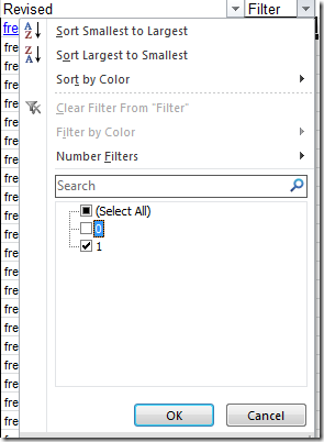
Then I added a simple filter to hide the correct results and only display those with differences.
I use this technique many times a week in comparing data lists.
Excel function of the week - AND
Thu, 23/12/2010 - 9:28am — jethroThe AND function takes each of the conditions inside the brackets and evaluates for their truth, and then multiplies the results together. TRUE = 1 and FALSE = 0. So if any condition is FALSE then the overall statement returns FALSE.
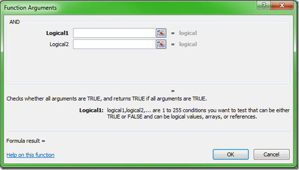
The formula for AND needs to be placed in brackets with each of the conditions separated by a comma. For example =AND(H1<1,G1>1)
In this instance the function will evaluate H1 to see if the value is less than 1. if it is then it will return TRUE or 1 and if not FALSE or 0. Then it will do the same for G1.
The two values are multiplied together and the answer is then either 1 or 0, TRUE or FALSE.
The Excel Help says:
One common use for the AND function is to expand the usefulness of other functions that perform logical tests. For example, the IF function performs a logical test and then returns one value if the test evaluates to TRUE and another value if the test evaluates to FALSE. By using the AND function as the logical_test argument of the IF function, you can test many different conditions instead of just one.
Relative conditional formatting in Excel 2007
Tue, 20/07/2010 - 8:23am — jethroI had a reader request some help with Conditional Formatting in Excel 2007.
Hi
Baffled in trying to get to grips with conditional formating in 2007
Scenario :
Column A = Actual Result
Column B = Target
Column C = Needs to show
1) If Actual result is less than 90% of target turn font colour RED
2) If Actual result is >90% of target and is <100% of target turn font colour AMBER
3) If Actual result is >= 100% of target turn font colour GREENIf column C meets criteria 1 use character "R", criteria 2 = "A" and criteria 3 = "G"
I can acheive 1 and 3 with =IF(a1b1,"G")) and then conditional format so that if contents of cell = R or G then colour font accordingly </B1,"R",IF(A1>
I`m stumped with the % factor and also think there might be a better way of doing it
Any help would be appreciated :)
Here is a solution to this problem.
We formatted two columns to give two examples as to how it could be done.
The actual column determines the percentage as part of the conditional format and formats in that way.
The result column formats on the “R”, “A”, and “G”.
 The formula in Column C1 is =IF(A2/B2<1,IF(A2/B2<0.9,"R","A"),"G") and this can be copied down.
Here are the rules for Column A


Recent comments
10 years 38 weeks ago
10 years 38 weeks ago
10 years 39 weeks ago
10 years 39 weeks ago
10 years 39 weeks ago
10 years 39 weeks ago
10 years 39 weeks ago
10 years 39 weeks ago
10 years 39 weeks ago
10 years 39 weeks ago