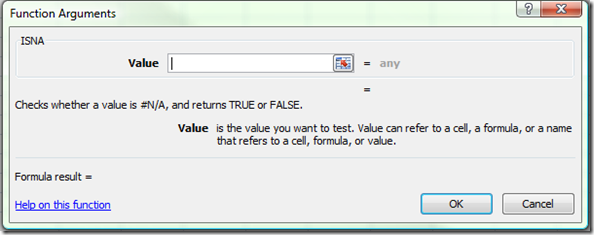
ISNA
How to remove #N/A errors in Excel
Fri, 14/12/2012 - 12:21pm — jethroToday I had an email request:
I wasn't sure how to post, or join so I'm sending my question to you this way. I cannot figure out how to remove the #N/A error in LOOKUP. If the cells are blank it returns the #N/A error - I'd like to return either a blank or 0 instead. How do I do that? Her is my formula. (I'm sure you can tell by my formula I'm a rookie at this.) Any help is appreciated. Thanks!
=SUM((LOOKUP(B6,{1,2,3,4,5},{40,30,20,10,0}))+(LOOKUP(C6,{1,2,3,4,5},{40,30,20,10,0})+(LOOKUP(D6,{1,2,3,4,5},{40,30,20,10,0})+(LOOKUP(E6,{1,2,3,4,5},{40,30,20,10,0})+(LOOKUP(F6,{1,2,3,4,5},{40,30,20,10,0}))))))
 I have written a post on this before when I explained the ISNA function.
In this case I will break down the first component of the formula and show you how to insert it.
First of all understand that because this formula is summing components that are lookups, if any one of them returns an error than the overall sum will be an error even if the rest is not an error.
So to fix =LOOKUP(B6,{1,2,3,4,5},{40,30,20,10,0}) when it displays #N/A (eg if B6 is less than 1) we would use this function:
=IF(ISNA(LOOKUP(B6,{1,2,3,4,5},{40,30,20,10,0}))=TRUE,0,LOOKUP(B6,{1,2,3,4,5},{40,30,20,10,0}))
The same concept could be used for each lookup component. In this case the formula would become very involved so there might be easier ways to do it. Sometimes breaking the individual components our into individual cells and then summing them is a way to give more visible results – and easily see which component is causing the error.
So Lois – i hope that helps – and thanks for liking us on Facebook!
Excel Tools and News from the web
Fri, 01/05/2009 - 11:01am — jethroI have had a bunch of pretty cool Excel things to post up – and finally got around to clearing my flagged items and browser windows.
Conditional Formatting
 I have written a couple of articles on Conditional formatting in Excel 2007 with lots of readers comments and requests for help. They are the two most read articles on this site.
I was very interested then to come across this article on Joseph’s site by Amit Velingkar where he shows you how to change the automatic colour ranges that are used in Excel 2007 for conditional formatting. He even includes some VBA code for this.
Excel Function of the week - ISNA
Wed, 03/12/2008 - 10:00am — jethroThe ISNA function is an Information Function. It is is used to return information about the status of a cell, or specifically another functions results. The most common use I have for this function is to validate the VLOOKUP function. If the VLOOKUP function is looking for a value that can not be found in the lookup range, then it will return #N/A as the result. Thus it is good to wrap that function in an IF Statement using the ISNA function to replace the #N/A results with something else – e.g. a text string such as “error” or maybe a zero.
=IF(ISNA(VLOOKUP(A1,$B:$B,1,FALSE))=TRUE,"error",VLOOKUP(A1,$B:$B,1,FALSE))
Remember the ISNA function returns a TRUE or FALSE. These equate to a 1 or 0 so can be used in formulas such as array formulas as well.


Recent comments
10 years 38 weeks ago
10 years 38 weeks ago
10 years 39 weeks ago
10 years 39 weeks ago
10 years 39 weeks ago
10 years 39 weeks ago
10 years 39 weeks ago
10 years 39 weeks ago
10 years 39 weeks ago
10 years 39 weeks ago