Spy Journal 3.0 Filtering the web for you

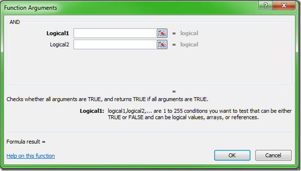
The AND function takes each of the conditions inside the brackets and evaluates for their truth, and then multiplies the results together. TRUE = 1 and FALSE = 0. So if any condition is FALSE then the overall statement returns FALSE.

The formula for AND needs to be placed in brackets with each of the conditions separated by a comma. For example =AND(H1<1,G1>1)

In this instance the function will evaluate H1 to see if the value is less than 1. if it is then it will return TRUE or 1 and if not FALSE or 0. Then it will do the same for G1.
The two values are multiplied together and the answer is then either 1 or 0, TRUE or FALSE.

The Excel Help says:

One common use for the AND function is to expand the usefulness of other functions that perform logical tests. For example, the IF function performs a logical test and then returns one value if the test evaluates to TRUE and another value if the test evaluates to FALSE. By using the AND function as the logical_test argument of the IF function, you can test many different conditions instead of just one.

Is that confusing? So are the backflips and name changes Microsoft have performed in this absolutely bizarre name changing fiasco.

Lets review shall we.

Live Mesh Beta - know to all users by the spinning blue circle, the blue folders in explorer, the 5GB of data and the sometimes very annoying conflict resolution process, (at least it had one) has been in use for the the last few years, and was touted as an awesome mobile, device rich, application development platform. People developed car stereo systems that synched playlists, mobile handsets that synched photos to their family from their phone, and many many people used it to share files and photos both between their friends and family and co workers and their own many devices.

I received this question on the website from Eric regarding conditional formatting:

Hi,

I have the same problem as a few people above but I don't think you got the point of the problem,

In xl2003 if you select A3:A9 and enter conditional format =B3 then select any other cell in the range it will show the conditional format for that cell e.g. A7 will show =B7

In xl2007 after following the same steps it will apply the correct formatting but if you select cell A7 to view the conditional format it will show as =B3. You get the same when checking any cell in range A3:A9.

This makes it near impossible to edit or amend or debug conditional formatting once entered.

Any advice would be appreciated.

Eric.

I started to post my answer and realised that i would be better off writing the whole thing as a blog post with some images to explain.

Hi Eric
i understand the problem and the first answer is that you cannot apply the same sort of logic between the two versions. The new versions (including 2010) manage conditional formatting completely differently, though some of the same concepts apply.
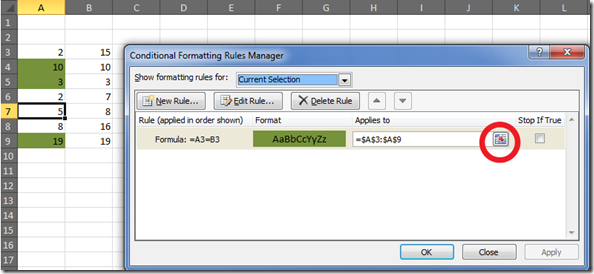
First of all your conditional format formula should be =A3=B3. This will apply the conditional format when the cell in A3 contains the same value as the cell in B3, and this will be relative - eg. when A7=B7 the cell in A7 will have the format applied. So you can see that the relative approach is correct in the conditional format manager in Excel 2007/2010
Second the problem you mentioned. When you look at the relative formula in cell B7 in excel 2003 it showed you just that formula. that is actually harder to debug if you think about it in Excel 2003 than in 2007/2010 as there is no way to see what other cells it also applies to. In Excel 2007/2010 the conditional format manager allows you to see the formula - and the range it is applied to and the little range box (circled in the image below) allows you to view this
The manager allows you to confine the selection to be evaluated to the selected cell(s), the current worksheet or other worksheets in the same workbook. If you then understand the relative / absolute nature of the formula you created then you can debug very successfully. I actually preferred this once I got a hang of using the manager to create sets of conditional formats than can be applied to multiple ranges simultaneously.

Outlook 2010 has some pretty sweet features. Here are some of the new ones.

Use the Outlook Social Connector with Facebook, LinkedIn, MySpace and Windows Live

Today, we are announcing that you can use the Outlook Social Connector with Facebook and Windows Live. Our partners LinkedIn and MySpace are also releasing updates for their providers. All of the latest providers appear on the provider page.

Download the social connector software

Download each of the social connectors

Choosing the right communication modality with the contact card