Conditional formatting in Excel 2007 - entire row colours
I had an interesting question about conditional formatting posed in the comments by Stephen.
In a new sheet, I am trying to make a whole row turn red, green or amber depending on the value of one cell in that row, so I can easily see which jobs we have won, lost or are pending. Any 'IF' conditional formula I write gets thrown out by Excel. What am I doing wrong?
I promised him an answer so here it is.
For this exercise I am making some assumptions.
- You are using Excel 2007 format Excel spreadsheet (.xlsx or .xlsm). These instructions will not work in detail for Excel 2003, though the concept is similar.
- That there are 3 conditions we are looking for. Of course Excel 2007 allows more than 3 conditions so you can add more if you need. (One of the improvements on Excel 2003 that only allowed 3 rules)
- That the entire row is needed to be coloured. If you need a smaller section than change the formulas accordingly.
- That the entire worksheet needs this formatting. If you need a smaller section than change the formulas accordingly.
- That the conditional formats are going to be based on a cell that returns a specific result based on some other rule.
The first thing I did was set up a spreadsheet using column H as my rule column. I often do something similar to this where I create a hidden column at the side of my data table and perform a IF function based calculation that returns me a value depending on the data evaluated. To use Stephens example I am assuming that jobs won have returned a 1, jobs pending returns a 0 and jobs lost a –1. These values can be anything – they are not relevant.
Now we are ready to create the conditional formatting rules.
The important thing to remember with conditional formatting when trying to work with more than just the selected cell is the absolute and relative cell selection rules. Read more about absolute and relative references if you need to.
Select the entire sheet (by clicking the gray triangle left of column A).
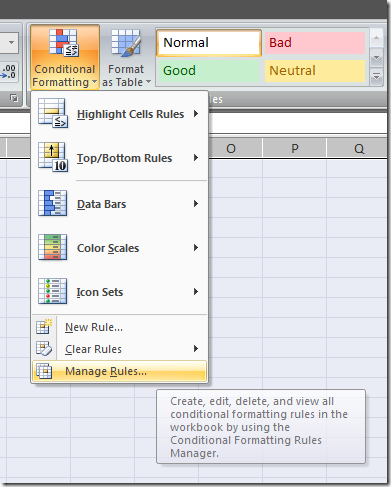
From the Home tab select the conditional formatting option and click Manage Rules.
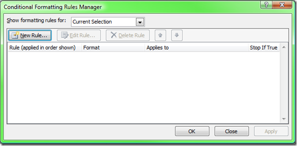
This brings up the Conditional Formatting Rules Manager.
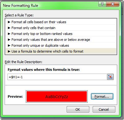
Select New Rule and then Use a formula to determine which cells to format.
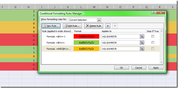
Create a rule where the formula is =$H1=-1 and the format is a fill of red.
Click OK.
Now make a new rule where the formula is =$H1=1 and the format is a fill of green.
Lastly make a new rule where the formula is =AND($H1=0,$H1<>””) and the format is a fill of amber. This rule keeps the cells unfilled where there is nothing in column H.
Click Apply to view the result.
The trick here is that the cell reference $H1 allows the rule to be applied down to every row and use the value in column H for every cell in that row.
Columns could be formatted in the same manner using a rule value in a row by locking the row and allowing the column to alter. eg. H$1.
Feel free to comment if this was helpful, or if you have other questions that need solving.


Comments
just change the number of
just change the number of columns in the range it works on to only work up to column N
is it possible to do with
is it possible to do with words like home /away for fixture lists, i want all our home games to be say blue and our away one to be green?!??!
tonyshand@hotmail.com
absolutely Tony the formula
absolutely Tony
the formula just needs to include the text you are looking for in quotes.
use a formula like this =A1="home"
Cheers
thanx.. it was really
thanx.. it was really helpful!! :)
Thank you thanks you
Thank you thanks you thank-you! I have had several excell spread sheets in excell 2003, and we recently switched to 2007. I have been searching the internet for hours, and no-one else's solutions actually worked. This one did! Thanks so so much!
Thank you so much! You
Thank you so much! You really simplified this whereas alot of other resources I searched through made it sound quite complex. Thanks again!
Years later (Fall 2010) found
Years later (Fall 2010) found this advice on Google and was a tremendous help. Thanks!
Hi there, Thanks for this
hi simon email the file to
hi simon
email the file to tim at spyjournal dot biz - ill have a look for ya
cheers
tim
Following the example you
Following the example you gave, how about setting a color on a row based on values on column "H" and another column, such as "G"?
I want to make a formula that makes the row green according to the following conditions:
=$H1<1 AND =$G1>1
Translation: For all rows showing values that are less than 1 (or show empty cells) on column H, but that show values greater than 1 on column G, make the rows green.
I know I have to use a formula with AND, but can't figure out how to do it. Would you have any ideas?
Thanks
Hi Jacques the formula for
Hi Jacques
the formula for AND needs to be placed in brackets with each of the conditions seperated by a comma. In your case =AND($H1<1,$G1>1)
The AND function takes each of the conditions are evaluated for their truth, and then multiplied together. TRUE = 1 and FALSE = 0. So if any condition is FALSE then the overall statement returns FALSE.
Cheers
Hi Tim, Thanks for having
Hi Tim,
Thanks for having this site, I appreciate the time people spend helping others. I know this thread is old, but I just started in Excel 2007. I like the 3 color idea. I have a bunch of projects that I have to track. Usually about 7 days in length. I track the start, due and actual completed dates. I was able to highlight them in a gantt style worksheet and get a date range establish, with the start at on cell and the due at the other, the cells inbetween are yellow. I used =AND(I$5>=$D6,I$5<=$E6). I5 to AM 5 is my date values. D6 is the first start date, E6 is the first due date. I wanted to have it turn "green" when it was completed, that value would be F6. I also wanted to have it turn "red" if it went past the due date in E6. I know I need to add 2 additional rules but was not sure how to keep the date ranges. I still need to have the start and due dates intact, just have the colors change based on the due and complete dates. Any ideas would be great. Thanks again Tim.
send me a sample spreadsheet
send me a sample spreadsheet and ill do it quicker than i can explain it - then you can see how to do it
cheers
tim at spyjournal dot biz
hi, in Excel 2007 I need to
hi,
in Excel 2007 I need to conditally format a row (fill with color) based on text rather than a numeric value. I have one worksheet and I need the rows highlighted with differernt color based on Approved,not approved, I can't seem to get the formula right to get the entire row highlighted. When I say "Approved " it only highlights that cell and not the entire row… Any suggestions pl let me know.
Hi Varun You need to check
Hi Varun
You need to check that the range that the formatting is applying to is more than just one cell. The formula will also need to have an absolute reference to the Approved cell. teg $A1. This will lock the condition on that cell for the entire row but stillbe able to be copied down rows and work for each row.
Hope that helps
Hi jethro, Your posts are
Hi jethro,
Your posts are really gold! I have a question about conditional formatting, can it work even if the value in the cell is a word? for example if the word ''Gone'' exists in any of the cells of ROW H, then the row should turn red. I tried inputing a new rule: as =$H1=''gone'' but this doesn't work while it works if i replace the word gone with a numerical value i.e. 3. Any ideas on how i can resolve this?
thanks
marina
Hi Marina the way i do this
Hi Marina
the way i do this is to create a separate index column that evaluates the words column with a rule to replace them with numbers - eg make a column that looks for "gone" and returns a 1 with an if statement - eg if(F1="gone, 1,0)
then i use the column with the values as the column to control the conditional formatting.
Cheers
Tim
I did this. I created a col
I did this. I created a col "DF" that read IF(DB2="Yes", 1,0). But it still works partially correctly. It highlights some of the "Yes" and some of the "No".
I applied the rule to col "A" to "DC". The index, "DF", is not in the range. Does this affect?
Thank you.
(Please delete, as I have
(Please delete, as I have solved this now)
Thank you! Have been stuck
Thank you! Have been stuck on this for a couple of hours - Microsoft Help no help at all - and following your instructions had it sorted within minutes.
awesome!
awesome!
Hi, Can anyone help me. Not
Hi,
Can anyone help me. Not sure if this is possible and my head is now hurting trying to think of a way this will work. Formulas in Excel are not my strong point.
I have a spreadsheet with staff names in column A, and Training Course Titles in Row 1.
If I put a date into say cell B2, I would like cell B2 to change to red after 6 months have elapsed to highlight that that person needs to refresher training.
Can anyone tell me the formula I need to use (if it is possible)
Thanks so much
Clare :)
Hi Clare this one is actually
Hi Clare
this one is actually quite easy to do
Select B2 and make a conditional format based on a formula. the formula needs to be =B2<(TODAY()+180)
that's making an assumption that 180 days is 6 months. and that the value in B2 is a date value.
note there is no $ around the B2. This can then be extended to all the other cells in this table.
Cheers
Tim
Hi Tim, Thanks for this. Ok
Hi Tim,
Thanks for this. Ok so when I put future dates in it works perfectly, unfortunately it turned my date red when it was only 2 days ago? Please can you advise whats wrong?
Many Thanks
Clare
my apologies - change the +
my apologies - change the + sign to a - sign
Cheers
Hi my problem is more or less
Hi
my problem is more or less the same as above but a little more complicated, actually i dont know why the conditional formating isnt working, it would be better if i can send you the file of excel so that you see the problem, but heres some info.
I have 4 columns, and X rows, in them they have some formulas that based in a number and in a word (some IFs by the way) you get a number, so that i can do the conditional formating that you posted above, the thing is that i cant get the formating, and i dont know why, my best guess is that the conditional formating isnt getting the number but instead is reading the other formula, i did try to put a word instead of a number in the column that you did with the -1, 0, etc. but with a word it didnt worked. well it kind of does but just with the cell that have the word not the entire row.
I dont know if i made myself clear, thats why i kind of need to send you the worksheet, ill be waiting for your responce, thanks a lot!!
Hi, just to simplify the
Hi, just to simplify the problem, the conditional formatfing doesnt work if you have a formula that results in the number that you need. For example if you move your numbers to the column G, and put in the column H, =G1 for example, the conditional formatting will stop working, and my best guess is that that happens because the conditional formatting needs a number and i have formula, or something... can you help me here, thanks!!
The initial problem is that i
The initial problem is that i need to color the rows of my worksheet based in two things, A text and a Number. In cell A1 you have the Date 11/11/11 in cell B1 you have 11/15/11 in cell C1 you have a Word for example Pending and in cell D1 you have the number 4 (its the result from the formula =DATEDIF(A1,B1,"d"). The rules are the next ones:
from 0 - 5 with text Pending you have the row in yellow
from 5 to 999 with text pending the row turns to red
If it turns rejected in cell C1 it turns to red whatever number is in cell D1
If it turns accepted in cell C1 it turns to green whatever number is in cell D1
but if it turn to number 7 it goes red.
Thats the whole problem i tried a lot of things, i can even send you my worksheet to see what i did, or you can do something based in the rules and example that i just post, i dont know im kind of desperate because nothing works... thanks a lot for your help.
Ignore the line "but if it
Ignore the line "but if it turn to number 7 it goes red"
Hi Luis for detailed requests
Hi Luis
for detailed requests for work like this we charge an hourly rate for work for clients. This site provides general advice and ideas to get you started. If you need us to work on a solution for you please email me at tim@spyjournal.biz. Our rates are US$120 / hour.
Cheers
Hi, and well its just a part
Hi, and well its just a part for a homework that i still dont know to do... but i cant afford 120 US/hour... so thank you very much, ill keep trying, thanks!!
I have been trying to figure
I have been trying to figure this out all night and maybe its just because I am not familiar enough with excel. I am trying to create a conditional formatting rule that I can easily copy to each individual column without having to rewrite the entire format. So kind of like duplicating a formula across a lot of columns. So in column A I want to highlight every number that is less than A2. But I want to duplicate this across all columns matching up to its own percentage B2, C2, D2. I can get one column to work with this formula =$A$3:$A$6<$A$2. Any Help would be great. Thanks
A B C D
76% 66% 76% 75%
67.83% 66.99% 74.27% 73.03%
66.92% 66.40% 74.35% 73.07%
66.79% 66.28% 74.27% 73.06%
66.76% 66.31% 74.34% 73.05%
66.94% 66.31% 74.23% 73.02%
67.02% 66.36% 74.25% 73.02%
pretty easy actually change
pretty easy actually
change your formula to =A$3:A$6
You rock. Exactly what I was
You rock. Exactly what I was looking for. Not the most intuitive of features.
Thank you so much! This
Thank you so much! This definitely helped a ton but I have another question. How do you count the number of cells are NOT conditionally formatted? I have a list of students and the number is constantly changing due to students adding and dropping the program. I've used the above technique to highlight the students that have dropped but I need a final count of students who are still currently in our program. Is there a function or something else I could use to count the cells that are NOT highlighted?
i would simply use the
i would simply use the reverse IF statement to the one you used to conditionally format the ones that are dropped and return a result into a cell - then filter on this column
hope that helps
Hi, I need your help in
Hi,
I need your help in replacing the conditional formatting placed on each cell of the workbook from red to yellow. Is there any way I can get it done in one go as manually it will be very time consuming.
Thanks & regards
Ruchi
Depends on what version you
Depends on what version you are using - both 2003 and 2007/2010 have a way to alter all the cells in a range that are conditionally formatted. neither are obvious. you can also use code to do it.
Does not work at all why i
Does not work at all why i did exactly same as on screen above.
Thanks a lot, Bro!!!!!!!!!!
Thanks a lot, Bro!!!!!!!!!!
This also works in Excel 2010
This also works in Excel 2010 no problems.
I have been struggling to use
I have been struggling to use this condition on an if condition that returns Due or Not due. Looking at you example which 1 is that you have in $H1? Excel doesn't seem to allow me select the whole column. =$H1=1
Hi, I have a certain sheet
Hi,
I have a certain sheet containing the day wise and week wise summary where in the day wise if the value is <=1 it should color RED, =2 it should colour AMBER, >2 it should color GREEN and in the summary if cell =15 it should color GREEN, <=5 it should color RED,>5but less than 15 it should color AMBER. Could u plz help.
Thanks this helps me lots
Thanks this helps me lots
I am trying to do this but I
I am trying to do this but I can't since the cell that is conditional formatting have a date and I don't know how to make a formula when the input in that cell is a date.
Day F S S M T W TH F S S M T
Day F S S M T W TH F S S M T W TH F
Date 24 25 26 27 28 29 30 31 1 2 3 4 5 6 7
john V V V V V V V V V V V V V
michle 8 0 0 0 0 4 8 0 0 0 0 0
tom 8 0 0 0 0 0 4 8 0 0 0 0 0
suresh 0 0 0 0 0 0 0 0 0 0 0 0 0
anthony 0 2 2 2 2 0
Please advise me how to make colour all fridays collum by using conditional formatting.
make a conditional format for
make a conditional format for the columns that looks for a value of "F" and applies it to the range of rows you need.
What I would really like to
What I would really like to accomplish seems so easy but trial and error is mostly error. I have a header and column fields that are auto filled based on certain criteria. I am trying to make a universal form as a timesaver. Ultimately, from A13:Q14 through infinity, a name is generated in column A. Each instance of generation will have a different number of names. I would like the borders of B:Q to auto fill when any text appears in A13 and south. As close as I've come has been =$13=ISTEXT(A13). The issue here is the borders are prefilled and as I add text, they disappear.
Dave