Conditional formatting in Excel 2007 - entire row colours

Fri, 19/09/2008 - 11:03am — jethro

I had an interesting question about conditional formatting posed in the comments by Stephen.

In a new sheet, I am trying to make a whole row turn red, green or amber depending on the value of one cell in that row, so I can easily see which jobs we have won, lost or are pending. Any 'IF' conditional formula I write gets thrown out by Excel. What am I doing wrong?

I promised him an answer so here it is.

For this exercise I am making some assumptions.

You are using Excel 2007 format Excel spreadsheet (.xlsx or .xlsm). These instructions will not work in detail for Excel 2003, though the concept is similar.
That there are 3 conditions we are looking for. Of course Excel 2007 allows more than 3 conditions so you can add more if you need. (One of the improvements on Excel 2003 that only allowed 3 rules)
That the entire row is needed to be coloured. If you need a smaller section than change the formulas accordingly.
That the entire worksheet needs this formatting. If you need a smaller section than change the formulas accordingly.
That the conditional formats are going to be based on a cell that returns a specific result based on some other rule.

The first thing I did was set up a spreadsheet using column H as my rule column. I often do something similar to this where I create a hidden column at the side of my data table and perform a IF function based calculation that returns me a value depending on the data evaluated. To use Stephens example I am assuming that jobs won have returned a 1, jobs pending returns a 0 and jobs lost a –1. These values can be anything – they are not relevant.

Now we are ready to create the conditional formatting rules.

The important thing to remember with conditional formatting when trying to work with more than just the selected cell is the absolute and relative cell selection rules. Read more about absolute and relative references if you need to.

Select the entire sheet (by clicking the gray triangle left of column A).

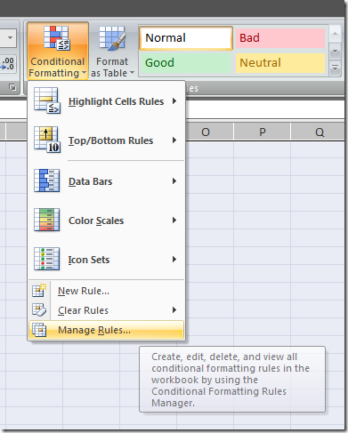
From the Home tab select the conditional formatting option and click Manage Rules.

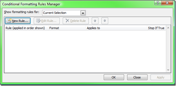
This brings up the Conditional Formatting Rules Manager.

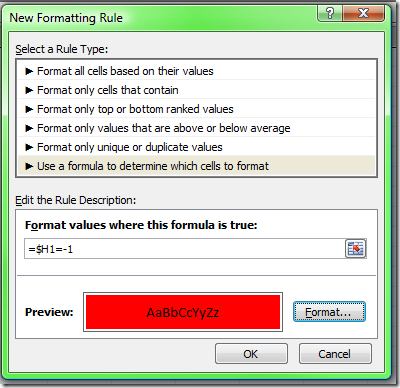
Select New Rule and then Use a formula to determine which cells to format.

Create a rule where the formula is =$H1=-1 and the format is a fill of red.

Click OK.

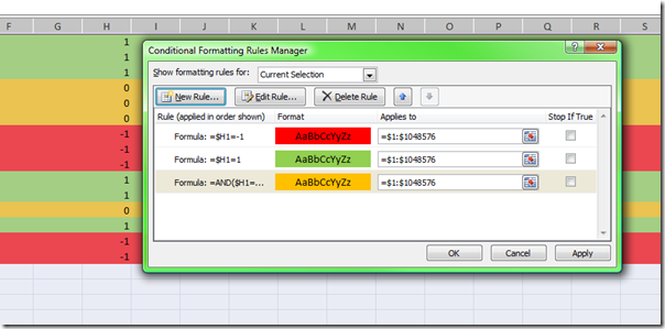
Now make a new rule where the formula is =$H1=1 and the format is a fill of green.

Lastly make a new rule where the formula is =AND($H1=0,$H1<>””) and the format is a fill of amber. This rule keeps the cells unfilled where there is nothing in column H.

Click Apply to view the result.

The trick here is that the cell reference $H1 allows the rule to be applied down to every row and use the value in column H for every cell in that row.

Columns could be formatted in the same manner using a rule value in a row by locking the row and allowing the column to alter. eg. H$1.

Feel free to comment if this was helpful, or if you have other questions that need solving.

Bookmark/Search this post with

jethro's blog
Login to post comments
251982 reads

Comments

Wed, 10/12/2008 - 4:27am — Anonymous (not verified)

Hi, Based on a cell value, i

Hi,

Based on a cell value, i want to the entire row to be set as "read only" row where no cells can be editable and highlight the entire row in grey color.

Is there a way to implement this solution in excel ?

Thanks in advance.
Regards,
Swami

Wed, 10/12/2008 - 8:23am — jethro

Hi Swami you would need to

Hi Swami
you would need to write a vba module to do this - a macro. you could write a function that looked for value changes but that would be very painful - the spreadsheet would check after very time a cell was changed and this would make using the spreadsheet very annoying.
here is one i wrote that does this - note the only point of locking a cell is if the worksheet is itself protected. otherwise it does nothing. It also assumes you have unlocked all the other cells in the worksheet.

Sub linechange()
If ActiveCell.Value = "lock" Then
ActiveCell.EntireRow.Select
With Selection
.Locked = True
With Selection.Interior
.Pattern = xlSolid
.PatternColorIndex = xlAutomatic
.Color = 7829367
.TintAndShade = 0
.PatternTintAndShade = 0
End With
End With
End If
End Sub

Wed, 10/12/2008 - 1:18pm — Anonymous (not verified)

Thanks for the quick response

Thanks for the quick response Jethro. Appreciate your time and help.

I was able to plug in the function and see the row getting highlighted. Part of my problem descripton earlier was not complete due to which the function might need few more changes.

I'm completely novice to excel programming and trying to learn.

The requirement is,
1. The cell values are selected based on a drop down list
2. When a value is selected say "Lock", the entire should be highlighted [This is happening as per your coded]
3. After highlighting the row, the row should be non-editable. With the above code, I could still edit the cell values are the row got highlighted.
4. If I select any other value other than "Lock" in the cell, the row highlighter should be removed and entire row should be editable again.

Is there a way to implement this ?

Again, thanks for all the time & help. It means a lot.

Regards,
Swami

Thu, 19/03/2009 - 3:47pm — Anonymous (not verified)

Hopefully you've figured this

Hopefully you've figured this out as the post was a long time ago, but just use a vlookup formula to put a number in a column next to the text, after you're finished hide the column.
The table array would have BrandOne with 1 next to it and so on, then write the rule to highlight the row, as previously demonstrated in this article, according to which number comes up as this will correspond to the text.

Thu, 19/03/2009 - 4:35pm — jethro

that will do it! thanks

that will do it!
thanks

Wed, 10/12/2008 - 1:37pm — jethro

Hi Swami did you note my

Hi Swami

did you note my point about the sheet needing to be protected?
see this post http://www.spyjournal.biz/exceltips/2006/05/protecting-cells-in-excel.html
cheers

Thu, 11/12/2008 - 1:28pm — Anonymous (not verified)

Yes, i did read the point

Yes, i did read the point about protected Jethro. By making the sheet procted, the whole of the sheet was locked rather than specific cell ?

Are we saying, if the excel sheet is not in protected format, there is no way to make a cell non-editable through macro ?

Next question is, is there way to hide the cell formulas from editing ? I was reading help and realised that it can be done by "protect / un-protect" option. If the excel sheet is not password protected, users will be able to unprotect the cell easily. Is there any other way to make the formulas hidden or non-editable by users ?

Appreciate your help.
Thanks,
Swami

Thu, 11/12/2008 - 3:45pm — jethro

Hi Swami you are correct - if

Hi Swami

you are correct - if the excel sheet is not in protected format, there is no way to make a cell non-editable through macro

protect the sheet and all locked cells are uneditable, and unlocked cells are editable

you can "hide" cells from editing several ways. whit text on white background, format with a custom format of ;;; or hide the row / column.
None of these actually stop the user from editing the cell however. The best way is to lock the cell and protect the sheet.

Cheers
Tim

Thu, 11/12/2008 - 8:18pm — Anonymous (not verified)

Thanks for the help Tim. Your

Thanks for the help Tim. Your inputs/solutions are extremely helpful.

One more question, in an excel book i have 2 worksheets names "Sheet-1", "Sheet-2". In "Sheet-1", i have data entered in say column 'A'. The same data of "Sheet-1" from Column'A' is populated in Sheet-2 of column 'A' using formula "=Sheet1!A1".

If i delete a row from Sheet-1, is there a way we could automatically delete the corresponding "Sheet-2" row as well. We can assume that "Sheet-1" and "Sheet-2" will have same set of rows with same data.

Appeciate your suggestions.
Thanks,
Swami

Thu, 11/12/2008 - 9:19pm — jethro

Hi swami there is a way -

Hi swami
there is a way - actually very simple - but very dangerous.
if you select 2 or more sheets (hold down CTRL and select the sheet tabs at the bottom) then any actions you perform will occur on each of the "grouped" sheets.
So inserting or deleting a row, typing in a cell etc will be repeated on every sheet simultaneously.
That is why this is also dangerous. If you forget to de-select the grouped sheets you can end up doing all sorts of damage
hopefully this helps you

Cheers
Tim

Thu, 11/12/2008 - 8:32pm — Anonymous (not verified)

Similarly in the above

Similarly in the above requirement stated, i would like to have a way to implement if we add a new row in "Sheet-1", the same row should be added to "Sheet-2" in same row number.

Fri, 12/12/2008 - 5:36am — Anonymous (not verified)

Just amazing Tim, You rock

Just amazing Tim, You rock !!...I can't stop thanking you for all help.

I could actually try your suggestion and see it working. I'm sure not many people would be aware of this feature :-)

Thanks again for everything.

Fri, 12/12/2008 - 5:21pm — Anonymous (not verified)

Hi Tim, Do you know if a

Hi Tim,
Do you know if a webservice API can be invoked from an excel macro or not ? If yes, how can we invoke it ?
Thanks,
Swami

Sat, 13/12/2008 - 1:07am — jethro

Yes you can - but

Yes you can - but unfortunately not one of my strong points. I have worked with people who did this sort of thing and then I edited the results they pulled back.
Bloomberg is an example - they use their own specific application to get data from their web servers and you can then manipulate that data in excel via a macro or formulas etc.

Wed, 17/12/2008 - 4:16pm — Anonymous (not verified)

Hi Tim, How can we implement

Hi Tim,

How can we implement a solution in excel for the below requirement ,

We have column A & B where column A has list values as "X", "Y". If users selects column A with value as "X", then Column B should display the valid list values as "1,2,3" and if user selects Column A with value "Y" the Column B should display the list of valid values as "6,7,8".

Appreciate your help.
Thanks,
Swami

Sat, 20/12/2008 - 12:47am — jethro

hi Swami this is a little off

hi Swami

this is a little off topic for conditional formatting
I am also very busy right now
how about you email me and we can talk about this

Cheers

Thu, 18/12/2008 - 3:09pm — Anonymous (not verified)

Hi Tim, Any suggestions for

Hi Tim,
Any suggestions for the above problem ?
Thanks,
Swami

Mon, 12/01/2009 - 1:08am — jethro

hi Swami this is a little off

hi Swami

this is a little off topic for conditional formatting
I am also very busy right now
how about you email me and we can talk about this

Cheers

Wed, 14/01/2009 - 9:39am — Graham Seymour (not verified)

Hi, I am using Excel 2007 and

Hi,
I am using Excel 2007 and am looking to use conditional formatting to change the colour of a row dependant on the numeric value in its right hand column - less than 80 (red), between 81 and 90 (amber) and greater than 90 (green). It is the 'between' formula (81 to 90) which I am struggling with. Are you able to help please?

Many thanks

Simmo

Wed, 14/01/2009 - 5:03pm — jethro

hi simmo you probably need to

hi simmo

you probably need to use an AND formula to help you.
you want both conditions to be true at once; that is the value needs to be greater than 81 and less than 90. heres the formula for cell A1
=AND(A1>81,A1<90)

Cheers

Thu, 15/01/2009 - 6:39am — Graham Seymour (not verified)

Many thanks Jethro -

Many thanks Jethro - struggled with this all of yesterday evening and you have now provided me with the means to get a good night's sleep!

Simmo

Thu, 15/01/2009 - 6:43am — Graham Seymour (not verified)

Thanks for your swift and

Thanks for your swift and very useful response Jethro - had struggled with that one all evening. Can now get a good night's sleep!

Cheers

Simmo

Fri, 30/01/2009 - 1:49am — FaeryKiss (not verified)

I followed your instructions

I followed your instructions regarding the conditional formatting, however instead of numerical values, I am attempting to use a value of Open or Closed for Column G. I'm having a bit of a struggle...... the formatting is not working at all and I'm wondering what I am doing wrong.

Thanks!
~FK

Wed, 30/09/2009 - 2:13pm — Anonymous

I had the exact same problem

I had the exact same problem and solved it by putting a space before Open. Aparently excel recognises Open as something else so it's an issue with the actual word. "Closed" however worked perfectly as per Tim's instructions.

Tue, 24/02/2009 - 8:22am — Mike (not verified)

Hi - thanks for the great

Hi - thanks for the great tips! I have a related question.

What if you want to shade a grouping of cells and not an entire row?

For example, If A1="Red", I want to shade cells b2:f3 red
If A4="Red", I want to shade cells b4:f5 red

I can get this to work if I only have one grouping, but if I have multiple groupings, each with their own color selection (A1 and A4), it doesn't seem to work.

When I select "Red" in A1, it turns all groups Red (b2: f5) and not just the first grouping and selecting the color in A4 doesn't do anything.

I am sure I could add separate rules for each grouping, but if I have 100 groupings and 3 colors for each one, that could be 300 rules to create and maintain.

Is there an easier way to do this?

Thanks,
Mike

Tue, 24/02/2009 - 2:00pm — jethro

Hi Mike you have the solution

Hi Mike
you have the solution - and as far as i know there no easier way.
you can try using the stop processing rules option after it gets a right result and see if that helps.
the other way to approach this is with formulas. create the logic you need in if statements in a row that you then hide - and base your conditional formatting on that.
eg for the first group have a formula that looks at the result in a1 and turns on a 1 if true and 0 if false. copy this across the sheet and then base your conditional formatting on the relative cell in that row. that way you only need one formatting rule and all the logic is held in the hidden row in a formula.
id be interested to see how you go with that.
Cheers
Tim

Wed, 04/03/2009 - 3:10pm — Zoran (not verified)

Appreciate this so much, I

Appreciate this so much, I had a hard time with it until I found this post. Cheers.

I love returning back to this site and reading the quality content you always have on offer.

Mon, 23/03/2009 - 11:52am — JimB (not verified)

I want to use conditional

I want to use conditional formatting to warn me if the sheet I'm working on is not protected. Is there a formula to flag that the sheet protection is on or off. The CELL function does not appear to do this. Reason for this request: I want to warn the user to be very careful with formulas if the protection has been accidentally left off in the last save. Regards Jim

Tue, 24/03/2009 - 11:46am — jethro

Hi Jim I could think of

Hi Jim
I could think of several ways of solving this but none really use the conditional format approach as the main way of achieving your aim.

This could be done by using a change state macro that then altered the value of a specific cell such that it could then be conditionally formatted. However this would mean creating the change state macro and it would run on every single change in the sheet and check the sheet protection status. this would cause the file to slow down and probably be unworkable. I don't think there is anyway to do it in the formula structure alone. You have already looked at the CELL function.

You could create a "test cell" that is supposed to be locked, and if its not use it to warn the user. I.e ask them to enter something in the test cell. If they can it will bring up a conditionally formatted warning.

The other alternative is to create an AUTO_OPEN macro that checks the sheet protection status and protects it if it was left unprotected. This is probably the best solution.

Cheers

Wed, 15/04/2009 - 1:58pm — Anonymous (not verified)

It seems as though everyone

It seems as though everyone is able to figure this out but me, HOWEVER... they are also basing their formulas off of a set value.

In my case, I am running a tournament and am trying to highlight an entire row based off the highest number in a Column.

I am able to highlight the CELL with the highest number in a Column (using this forumla "Formula Is =G96=MAX($G$92:$G$101)" ,but I can't get the ROW that corresponds with the highest number to highlight.

Anyone able to help?

Thu, 16/04/2009 - 1:50pm — jethro

hi this was pretty simple

hi
this was pretty simple once i figured it out
i added my data in column E
I selected an entire row - eg row 4
i added a rule as follows
formula =$E4=MAX($E:$E) and made it apply to =$4:$14

what this does if you think through the steps is that for every cell in the row 4 it looks at cell in column E (where my values are stored) and if the cell in the current row is = to the max of the cells in column E then it applies it to every cell in that row.

Hope this helps
Cheers
Tim

Tue, 28/04/2009 - 10:57pm — Allie (not verified)

Hi, First I would like to

Hi,

First I would like to help you for all the help you have unknowingly given me already, you have been very helpful in guiding me through the quagmire that is the new Excel!

I have followed your wonderful instructions so far and they have worked a treat, however I am trying to get it so if a number is >90 or <75 to highlight using the conditional formatting, however Excel does not seem to want to allow this.

Could you possibly help me?

Thank you

Allie

Wed, 29/04/2009 - 5:41am — jethro

Hi Allie Thanks for your

Hi Allie

Thanks for your comment
Try using a conditional format with a formula like this one =OR(F6<75,F6>90)
where F6 is the cell you are wanting to operate on. By making sure there are no $ in the formula if you copy this format to any other cell it will remain relative.

Cheers
Tim

Tue, 05/05/2009 - 3:51am — Aaron (not verified)

I can sleep again!! I have

I can sleep again!! I have been struggling with this for about 3 days. And google finally gave me a link that worked. Thank you so much!!!

Tue, 05/05/2009 - 8:57am — jethro

glad you can get some sleep

glad you can get some sleep now!
cheers for the comment Aaron

Sat, 20/06/2009 - 2:56am — Anonymous (not verified)

I tried the example but in my

I tried the example but in my spread sheet some -1 and 1 are getting highlighted in red colour while Iam applying condition only to -1

Sat, 20/06/2009 - 8:04am — jethro

only some? want to send me

only some?
want to send me the spreadsheet?
email tim at spyjournal dot biz

Fri, 03/07/2009 - 12:14am — Premal Matalia (not verified)

Thanks a lot... I was

Thanks a lot... I was strulling for days.....
It helped me a lot

Tue, 11/08/2009 - 4:00am — Anonymous

Hi, can this solution be

Hi, can this solution be implemented on all Sheets in the Excel Spreadsheet? Thank you very much....

Wed, 23/09/2009 - 11:16pm — Anonymous

Good tips for begginners like

Good tips for begginners like myself

txs

Tue, 06/10/2009 - 7:03pm — Anonymous

Last formula don't work here,

Last formula don't work here, I need ; instead of ,. Like this:
=AND($H1=0;$H1<>"")

Wed, 11/11/2009 - 5:33am — Anonymous

HELP ME before I pull

***HELP ME*** before I pull out all of my hair ;o) Being female this would not be pretty!!

I am working in a large company and we are upgrading all machines to Vista. Part of this is opening tickets for issues raised during upgrade. So I log the ticket on a certain date

Column F Column G
Ticket logged ticket open/closed
12.10.09 open
14.10.09 closed
I have applied a conditional format to column G to change colour of cell if ticket 'open' (based on 'containing text' rule) What I am trying to do is.....in the ticket logged (column F) i need the box to be red if date logged for more than 2 days before ticket being closed off (action-ed). how do i do this??

Fri, 13/11/2009 - 10:10am — jethro

you need to have the dates

you need to have the dates ticket logged and closed in separate columns - F and G
then you can perform a calculation of the more than 2 days scenario and that can be used to action the conditional formatting
its fairly simple math
so in column H create an if statement =IF((F2+2) "less than" G2,"late","on time")
then use the conditional formatting based on the text in cell H being "late"
( replace "less than" with the less than symbol)
Hope that helps

Fri, 15/01/2010 - 7:18am — Anonymous

Hi I tried your formula but

Hi I tried your formula but Excel is highlighting rows that are not fitting my criteria. I have the formula pointing to a cell that has a series of numbers and I want to highlight the row when that cell (first one is S2) is >540. When I apply the formatting, it highlights ramdom rows, some greater than 540 and some less than. I figured it might be a cell format issue but no luck thus far

Wed, 17/02/2010 - 7:51pm — Anonymous

Thanks so much it really

Thanks so much it really worked well for me :)

Fri, 23/04/2010 - 5:34am — Anonymous

Hello, I want to higlight

Hello,

I want to higlight entire row when a particular text is on the cell, ( is there something which can allow us to give date and time, when that formating is happening?)

I would appreciate your help.
I can be reached at lav_at_21@yahoo.co.in.

Thanks
Lav..

Fri, 07/05/2010 - 5:56pm — jethro

Not using conditional

Not using conditional formatting - you would have to run an on change event using VBA code.

Fri, 14/05/2010 - 10:44am — Anonymous

Thank a lot that worked for

Thank a lot that worked for me... now i have one more question.
I have a sheet(baby sheet) with columns till I (I is cell the cell where status is updated with drop down as pending and complete) what i need is when ever there is any thing selected in cell I whether pending or complete, i want to copy entire row of column and paste it another sheet which is master sheet.. whenever there is any update in the baby sheet the data should be copied to master sheet.

Thanks
Lav :)
lav_at_21@yahoo.co.in

Mon, 17/05/2010 - 1:58pm — jethro

You would need to write some

You would need to write some fairly complex VBA code to do that - and once again call it with an on change event. Not something I can explain in a comment!

Thu, 29/07/2010 - 2:31am — Anonymous

Hi, Is there a way to limit

Hi,

Is there a way to limit the number of columns it highlights - i only need it to highlight up to column N.

Thanks
Daniel

Site Construction and Maintenance by Jethro Consultants

Gidday
Glad to have you stop in.
I write about my family, the internet, technology and gadgets, productivity with Microsoft Office applications Excel Tips and more.