Spy Journal Excel Tips

Tuesday, May 31, 2005

Summing time in Excel

ExcelTip.com has this great tip.

Summing time values that are separated into hours and minutes in different columns
Problem:
Columns B:C contains numbers representing hours and minutes accordingly.
How could we sum up the numbers in both columns to a single time value?

Solution:
To get a time value representing the sum of hours and minutes in columns B:C
use the following Array Formula: {=SUM(TIME(B12:B14,C12:C14,0))}

Example:

Hours___Minutes
5_______20
6_______50
3_______10

Result: 15:20
Formula: {=SUM(TIME(B12:B14,C12:C14,0))}

Notes:
To perform an Array Formula: Insert the formula, press F2 and then press Ctrl+Shift+Enter simultaneously.
The format in the cell contains formula is:[HH:MM]

Monday, May 30, 2005

Using the CELL function in Excel

Finding the full filename and path for any given file can be done fairly simply using the CELL function.
Using =CELL("filename",C5) will return the full path, filename and sheet name.

Extracting the specific information of the file name and path is a little more difficult but can be achieved using the text string functions LEFT, MID, FIND and MID
To get the full path and file name use =LEFT(CELL("filename",C5),FIND("]",CELL("filename",C5)))

To get the file name only use =MID(CELL("filename",C5),FIND("[",CELL("filename",C5))+1,FIND("]",CELL("filename",C5))-FIND("[",CELL("filename",C5))-1)

To get the path easily use the combination of the above two cells listed as cells C20 and C21 respectively =LEFT(C20,LEN(C20)-LEN(C21)-2)

Thursday, May 26, 2005

Clarification

Yesterday I wrote a post about using screenupdating and displayalerts. I obviously didn't make it very clear how to do this.

Jon Peltier wrote the following:
I think you mean:

Application.ScreenUpdating = False
Application.DisplayAlerts = False

at the beginning, and

Application.ScreenUpdating = True
Application.DisplayAlerts = True

at the end of a macro.

The use of VBA arrays rather than the worksheet cells is definitely a huge time saver.

Another big timesaver is to avoid selecting an object before then doing something with the selection object.

For example, replace

ActiveChart.PlotArea.Select
Selection.Width = 250

with this

ActiveChart.PlotArea.Width = 250

BTW, both the Contextures.com site and my PeltierTech.com site now feature RSS feeds. Not a big deal, since I update mine about every two weeks.

- Jon

Thanks a lot Jon for that helpful stuff.

Wednesday, May 25, 2005

Speeding up VBA macros in Excel

Here are some simple methods to speed up how fast macros run.

Application.ScreenUpdating = True
Use this command at the beginning of a macro with True and at the end as False. When the macro runs the screen will stay static. The pc can run the macro faster as it doesn't have to refresh the screen as the macro changes sheets, workbooks or recalculates.

Application.DisplayAlerts = True
Use this command when the macro you are running will require user input that you need the default answer to. Eg if you are saving a file using the ActiveWorkbook.SaveAs command and the file already exists. This means the user won't have to react to the beep and the onscreen dialog box thus shortening the total running time.

Use Arrays instead of operating directly on the spreadsheet.
If you need to manipulate a set of data on a sheet, it is often better to select that data as an array in memory, use if then and for next and do while loop statements to process the information, then when it is complete paste it back into the spreadsheet. On small data sets, say a couple of thousand cells this won't make a hugely noticeable difference, but on a sheet with tens of thousands of cells this will make a huge difference.

References to previous array posts

Tuesday, May 24, 2005

SUMPRODUCT Array formula

Here is a SUMPRODUCT array formula.
=SUMPRODUCT((A2:A11={"A"})*(B2:B11<>{""})}
You need to press CTRL SHIFT ENTER when editing to save this formula. That will put the {} brackets around it,. Ypu do not need to type these.
This formula will count all the items in the list that have an A in column A and do not have a blank in column B. Obviously you can change the criteria to what ever you need.
This is probably the best way of calculating this sort of thing.

Thursday, May 19, 2005

Mark beat me to the follow up post on splitting out names without formulas by providing the formulas.
He has kindly separated them out so you can see the individual components. As he mentions the FIND Formulas can be integrated into the names formulas.

Tim,
I thought this might be of interest to you and your readers.
Obviously the logic could be extended if you had more than 3 names possible.
You can try to put the formulas for 1st & 2nd space into the formula for each name, but the formulas start to get very scary.
Another tip too with this type of data if there is any possibility of having more than one space between the names, use the TRIM function to eliminate extra spaces.
In the example you gave to overcome the possibility of extra spaces, make sure the 'Treat consecutive deliminators as one' box is checked.
Mark

Names.xls file attached.

Wednesday, May 18, 2005

Splitting first and last names in Excel

I received an email from ExcelTip.com the other day that explained how to separate a column of first and last names into two columns, first and last separately. I knew how to do it conceptually but had never bothered.
Anyway today I was asked that very same question and I was able to explain!

Select the column with the fullnames in it making sure there is an empty column to the right.
Select Data | Text to Columns.
Select Delimited in step 1 and Click Next
Check the space checkbox in step 2 and click Finish.
Voila!

Monday, May 16, 2005

Rounding to nearest 5 cents part two

Well after posting my really complicated solution to the question about rounding to the nearest 5 cents I got given a whole bunch of alternative solutions. (Mark I'm disappointed you didn't have a better one for me!)

Try these:
=ROUND(price*(1+markup)/0.05,0)*0.05
=ROUNDUP(price*20*(1+markup),0)/20

Both of these mathematically do essentially the same thing, though the different functions give different results with ROUNDUP always rounding up where as ROUND is a 2/3 rounder.

=CEILING(price*(1+markup),0.05)
This will always round up to the nearest 5 cents.
=FLOOR(price*(1+markup),0.05)
This will always round down to the nearest 5 cents.

Tuesday, May 10, 2005

Design and layout presentation tips for Excel

The first 6 months that I worked as a consultant, I worked with a team of consultants. I received a lot of experience in many different industries rapidly. The head consultant taught me some skills that I have never forgotten. Most of these relate to appearance and presentation.
When completing a job for a client, whether it be a financial reporting system, a database, a chart or just a timesheet I always remember what I learnt about presentation. The head consultant would annoy me by spending inordinate amounts of time (or so I thought) on fussy little details, like colour matching, lining up boxes and graphs, font sizes and colours etc. However I quickly learnt from him that making a bad job look good helped sell it to the client. While I hope I haven't learnt his ethics, I did learn that making the job look good earns brownie points like you wouldn't believe.
Here are some of the tips and hints I learnt from him.
Design and layout
One of the easiest ways to set up spreadsheets that calculate or generate results that need to be reported is to separate the function from the form. Just like a shiny exterior on a car hides the internal engine and wiring. I always create my reports and front end menus to look good and generate results and calculations in more functional sheets.
Hiding unnecessary sections
If you must have calculations and working sections visible, then hide the unnecessary bits. Hiding a row or column is only one way of doing this. Using the group function you can rollup whole rows of information, eg components that add to a subtotal or constants and variables such as exchange rates, interest rates, and other indexes. Additionally you can use the ;;; format of a cell rendering the cell contents invisible. Finally colour can be used. Make the background and font the same colour. The danger with these last two approaches is that well intentioned people (users) may delete these seemingly blank rows or columns. If you do this then use cell protection.
Use of colour and graphics
I like to use the company logo or other graphic as a design element in my spreadsheet. Sometimes I do this by using the corporate colours, other times by using the graphic itself. If I have a spreadsheet with a lot of macro buttons, I may use command objects and use the logo as a picture on the button. Beware of using large bitmaps as this will increase file size. The background can be a picture also if the content (and font colours) can be easily displayed. Editing the picture in Photoshop or other graphic editing program you can reduce the brightness and contrast to get a faded picture that can make an attractive background. Alternatively use the corporate colours in background with an accenting colour (usually darker) as the font colour.
Removing excel components
There are a number of excel components that you can turn off. Menu screens and reports screens may not need horizontal or vertical scroll bars, sheet tabs or row and column headings. Using macro buttons to return to a menu can overcome the need for sheet tabs. Not displaying gridlines will give a clean uncluttered look to a layout, and then using borders as necessary can create emphasis in the right areas.
Fonts
Do NOT over use fonts. Every design shop, course or artist will tell you this. I tend to use only one font for an entire spreadsheet, or one for the presentation and the standard Arial font for working sections. Choose a font that reflects the type of spreadsheet, keep the quirky fonts for fun and light stuff not board room presentations. Use bold and italics sparingly.

Thursday, May 05, 2005

Dynamic line graphs that work with zeros in Excel

I make a lot of graphs for financial reporting for clients. In most cases these are made in database type files that have monthly data imported from a large accounting system. In most cases I need to produce line graphs that will take the whole years results, but only show up to the current month.
The main problem with this is that if you have a line graph for 12 periods, but you only have values in the first 3 months your line will go up and down for 3 months and then for the remainder of the year go down to the x axis and stay there. See figure 1 for an example.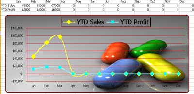

The best way I have discovered to resolve this is to use #N/A errors deliberately.
In most cases the file will have a current month selected. I use this for report headers etc. It is also used for the graphing.
Using a formula similar to =IF(monthdate>currentdate,#N/A,data) I can generate #N/A errors deliberately for the months where I have no data.
#N/A never shows up in a graph. Thus we have created a line graphs that can be dynamically updated. See figure 2.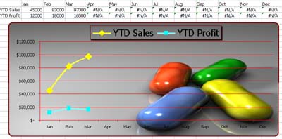

Wednesday, May 04, 2005

Rounding to nearest 5 cents in Excel

A reader sent me these two questions.

For school tuckshop - they have cost and sell prices and need a formula to work out what percentage they have added on to cost to get sell price for each item.
They need to figure out what percentage they are charging for each item – it is not uniform and they are trying to work out what they were doing so they can put correct process in place.

Can you also remind me what the "rounding up" formula is? It has been a few years since I did it and I wanted to round up to the nearest 5 cent.
Cost plus 40% rounded to nearest 5c is = ((cell name * 1.4) ROUND *.5)
Have I come anywhere near close???

The first one is actually very easy
=(sell-purchase)/purchase

The second is a little harder
Rounding to the nearest decimal point (eg 10c) is easy using the ROUND function.
=ROUND(B12*(1+markup),1)
The ROUND function uses the number of decimal places you want to round to . Using positive numbers rounds to the right of the decimal point, using 0 rounds to a whole number, and using negative numbers rounds to decimal places to the left of the decimal point.

However rounding to the nearest 5 cents is a bit more complicated.
In the following formula I have used the MOD function. This function gets the remainder after dividing by a number. In this example I have looked for all results where the remainder is 1 or 2 (any number that ends in 1, 2, 6 or 7) and then subracted the remainder from the result to get a number that ends in either .05 or .00
Wherever the remainder is 3 or 4 I have rounded up by adding the remainder
=IF(MOD(cost*(1+markup),0.05)<3,cost*(1+markup)-MOD(cost*(1+markup),0.05),cost*(1+markup)+MOD(C14,0.05))

I have attached a sample workbook. Right click and Save Target As to download.
price rounding exercise.xls

Monday, May 02, 2005

Using the COUNT functions in Excel

There are several COUNT functions in Excel. Here is a brief explanation of each and when to use them.

COUNT(value1,value2,...)
Use the COUNT function to count all the numbers is a range or multiple ranges. Each cell with a number in it returns a count of 1.
Value1, value2, ... are 1 to 30 arguments that can contain or refer to a variety of different types of data, but only numbers are counted.
COUNT only counts numbers. If an argument is an array or reference, only numbers in that array or reference are counted. Empty cells, logical values, text, or error values in the array or reference are ignored.

COUNTA(value1,value2,...)
If you need to count logical values, text, or error values, use the COUNTA function.
Value1, value2, ... are 1 to 30 arguments representing the values you want to count. In this case, a value is any type of information, including empty text ("") but not including empty cells. If an argument is an array or reference, empty cells within the array or reference are ignored. If you do not need to count logical values, text, or error values, use the COUNT function.
Each non empty cell returns a count of 1.

COUNTBLANK(range)
Use COUNTBLANK to find the number of empty cells in range.
Cells with formulas that return "" (empty text) are also counted. Cells with zero values are not counted.

COUNTIF(range,criteria)
Use the COUNTIF function when you you want to see how many of a specific value exists in a range. Eg the number of times a name appears in a list of names.
COUNTIF counts the number of cells within a range that meet the given criteria.
The criteria is in the form of a number, expression, or text that defines which cells will be counted. For example, criteria can be expressed as 32, "32", ">32", "apples".

Additional information.
Microsoft Excel provides additional functions that can be used to analyze your data based on a condition. For example, to calculate a sum based on a string of text or a number within a range, use the SUMIF worksheet function. To have a formula return one of two values based on a condition, such as a sales bonus based on a specified sales amount, use the IF worksheet function.

Copyright Notice. All documents and text contained in this web site www.spyjournal.biz and sub pages is copyright material of Jethro Management (c) 2004 unless noted as being copyright material of someone else. No public reproduction of the content on this site in any form is permitted without express written permission.

Unless otherwise expressly stated, all original material of whatever nature created by Tim Miller and included in this weblog and any related pages, including the weblog's archives, is licensed under a Creative Commons License.