Monday, January 31, 2005
Protection in Excel Spreadsheets
I generally look at up to 4 levels of security on an Excel file.
At the end of the day there really isn't a heck of a lot of security for those who know how to remove protection from files. However for general users who are unaware of this here is how I do it.
The first level of secuirity is to make a file read only, and require a password to open or access the file.
The second is to require another password to modify the file.
Third inside the file you can have various levels of protection controlled by macros. Lock the entire file up and then require users to use password controlled macros to unlock various portions of the file.
Fourth allow access to the whole file with a master password (or use the vba project password to inhibit access to the macros).
I will provide the VBA code for the password protection (third level) macros later.
Saturday, January 29, 2005
Changes to selecting all cells in Excel 2003 from previous versions
CTRL A is the shortcut (common across most Microsoft Products) for selecting all. In an excel spreadsheet it selects all the cells in the sheet. (All 16,777,216 of them!)
However there has been a slight change in Excel 2003 from previous versions as to how this works. Now it is a two step process. The first time you select CTRL A it will select the current region (which may be the entire sheet) and the second time you press CTRL A you will get the entire sheet. This can be a trap for the unwary if you are used to using the shortcut without looking at the screen.
If there is no data in the sheet then CTRL A will get the entire sheet and if the selected cell(s) is not adjacent to or inside any regions (cells with data in them) then you will also get the whole sheet first time.
The other method of selecting the entire sheet by clicking the box left of column A and above Row 1 still works as before.
Thursday, January 27, 2005
New Zealand Excel Website
I have found a new excel website (actually Rob had the answer for the strange formats in Excel).
Robs Excel Resources WebSite has plenty of VBA code available for all sort of useful things like finding broken references and rounding up and down, as well as plenty of other useful tips and hints. Note: this site doesn't appear to work in Firefox. Worth bookmarking all the same.
Trick custom formats in Excel
As a follow up to the entry about custom formats here's a formatting trick Mark discovered a few years ago.
Format a cell with a custom format of \bill,
Now enter any number in this cell. Positive numbers or results of formulas will return bill while negative numbers will give you -bill.
Try other variations using the \ in the front. I am not sure why or how this works or what the logic is for some text giving different results. For example \gra will work but \grant won't. \time returns ti11900.
If anybody knows why this is so please let me know! Add a comment so everybody else can find out too.
Don't forget you can be added to the email list if you want. The subscribe to the daily email link is in the side bar.
Monday, January 24, 2005
Arithmetic Operations in Excel
In Excel the normal mathematical order of operation exists in formulas. That is that arithmetic operators are processed in the following order, and internal nested brackets treated first.
^ to the power of
* multiply
/ divide
+ plus
- minus
So remember when making a formula that involves multiple operators that you use brackets where necessary.
For example 24/2+4 = 16 but if you wanted the answer to be 4 then you would need to use 24/(2+4).
Thursday, January 20, 2005
Customise the toolbar in Excel
From Excel Tips
Almost 50% of the menu bar line is empty.
Use this empty space to add useful icons such as Page Setup, Custom Views, Macro, and more.
To add icons to the menu bar:
1. Place the mouse arrow on one of the toolbars, right-click, and select Customize from the shortcut menu.
2. Select the Commands tab.
3. From Categories, select File and drag the Page Setup icon to the menu bar.
4. Repeat step 3 for the Custom Views icon (from View) and for the Macro icon (from Built-in Menus).
5. Click Close.
Note:
These new icons also have keyboard shortcuts, which are used by pressing Alt and the underlined letter.
For example, to open the Page Setup dialog box, press Alt+U.
Screenshot
Wednesday, January 19, 2005
SUMIF Formula in Excel
The SUMIF formula is a very powerful tool for analysing data.
It allows users to identify subtotals in a range using a criteria that you set.
For example a range of salary data containing names and weekly pays in two columns A & B.
Using SUMIF you can simply and easily calculate the total pays made to any employee.
The SUMIF formula uses the following syntax.
=SUMIF(criteria range, criteria, sum range). The sum range and criteria range can be the same if necessary.
Usually this would mean that you would write the formula for our payroll example above as follows:
=SUMIF(A:A,"name",B:B)
You can replace the "name" with a cell reference to an input cell (or a named range) thus allowing users to change the name or even use data validation to create a drop down list of potential names.
As an auditing tool in this instance it is useful as well.
Creatg a table of the unique employee names and add the formula beside each. The total of these individuals' pay totals should equal the total of all pays in column B. If not then there is either an employee name that hasn't been added to your summary table, or there are typing errors in column A, Eg spaces before or after a name etc.
CTRL SHIFT ENTER (CSE) Formulas in Excel
There are a bunch of things you can do with array or CSE formulas in Excel. These include reducing the number of formulaic steps required to achieve a result. For example take a column of data C1:C20 that has a number of calculations in it. Some of these return errors. One way to calculate the number of errors is to create a second column (say D) that has a formula returning a result , eg 1, if there is an error. A sum of this column will tell you how many errors there are.
Or you could use a CSE formula like this one. Note when entering this you must press CTRL SHIFT ENTER to finish editing the formula. This will put the {}braces around the fomula. You don't need to type these.
{=CONCATENATE("There are "&SUM(IF(ISERROR(C1:C20)=TRUE,1,0))&" errors","")}
Sunday, January 16, 2005
Limiting the Movement in an Unprotected Sheet
From Excel Tip of the Day
In this example, the sheet is divided into two parts: an area where movement is allowed (the Scroll Area), and an area where movement is restricted (that is, a protected area), without protecting the sheet.
Set the Scroll Area range in the Properties dialog box:
1. Click the Properties icon OR From the Control Toolbox toolbar, click the Properties icon.
2. In the Scroll Area text box, type the scroll area range, or type the defined Name for the range (this is flexible, if you plan to add more data to the range, it is better to use a defined Name).
3. To cancel the Scroll Area restricted range, clear the Scroll Area text box.
Note:
You cannot add two Scroll Areas to the Scroll Area text box.
View screenshots
Friday, January 14, 2005
Top Ten Excel Annoyances
Curt Frye lists the top ten annoyances as gathered from a small survey he conducted. He then presents the answers. Curt is the author of a book Excel Annoyances.
I have listed the first 3 here for you. Follow the link for the rest
1 Format part of a cell's contents
2 Add a carriage return to a cell's contents
3 Insert or delete a single cell
4 Delete a formula and keep the result
5 Add text to a displayed numerical value
6 Display partial hours as a decimal number
7 Prevent copied formulas from changing cell references
8 Create a named range from multiple sheets
9 Copy charts as pictures
10 Speed up recalculations
Format Part of a Cell's Contents
This one is so easy, you'll kick yourself when I tell you. To format part of a cell's contents, click on the cell to display its contents in the Formula Bar just above the worksheet and below Excel's toolbar. Select the characters you want to format in the Formula Bar, and use the buttons on the Formatting toolbar to change the characters' appearance. This solution might seem basic, but you'd be surprised how many folks think it's impossible to edit part of a cell's contents. The program sure doesn't make it obvious.
Add a Carriage Return to a Cell's Contents
You can add a line break inside a cell by pressing Alt-Enter. Yep, that's all there is to it.
Insert or Delete a Single Cell
Have you ever typed in a data list, only to discover that you left a value out of the middle? Sure, you could just cut and paste the data below the item you missed and type it into the blank cell, but here's a quick way to add a new cell in the middle of list without cutting and pasting.
Thursday, January 13, 2005
Custom Formats in Excel
Excel allows you to format cells with a wide vareity of standard formats. However there is often a time when you need to customise a format. Examples can include adding leading zeros to numbers for a consistent result, special date formats, hiding data etc.
How to customise a format.
Select the cells you want and then click Format Cells and choose the Number Tab. In the bottom of the left section of format categories select Custom.
A wide range of pre generated custom formats will appear. You can actually modify one of these or add your own. The good news is that the custome formats you create stay with the spreadsheet on any pc. The bad news is that custom formats made in one spreadsheet won't be available in this list in another spreadhseet.
Three examples
Adding leading zeros to a range of 3 and 4 digit numbers.
Type 0000 in the box under the word Type on the right hand side of the format dialog box. Now 397 will display as 0397.
Hiding data in a cell.
Type ;;; in the Type box. No matter what colour font or cell background you cannot see the data in this cell. The data or formula can still be edited in the formula bar.
Special Numbers.
Red bracketed negative numbers, two decimal places, leading spaces before the numbers and the $ at the far left (with a space), two spaces at the right edge and commas at thousands.
$* #,##0.00 ;[Red]($* #,##0.00) ;
Note I have added an extra space to the non negative numbers so that the digits will line up with the negative ones. Also make sure you get the space at the beginning before the first $.
As you are fiddling with the custom format it displays a sample of the result.
Tuesday, January 11, 2005
See through shapes in Excel
This is a go and see entry. Andrew's Excel tips has posted an excellent article on how to create apparently transparent shapes on an excel page.
These can be used for all sorts of effects including 3 dimensional objects, and buttons and other pictures. They can also be used in graphs to make a graph appear embedded in another picture.
Monday, January 10, 2005
Adding trendlines to Charts in Excel
Excel has the ability to create automatic trendlines in charts. Simply select any series in a chart and right click it. Choose the option Add Trendline and a dialog box will display with all the different trendline options available. After selecting one it will appear on the chart. You can then edit its colour, line weight by right clicking the trendline and choosing Format Trendline.
Saturday, January 08, 2005
Exporting Excel files to a CSV or TXT (tab delimited) file
Excel enables you to save a file in a number of formats.
A text or csv file is also known as a flat file. The reason for this is it is a 2 dimensional database only.
This means that only 1 sheet can be saved in the file.
The sheet must consist of columns and rows (fields and records) of data.
Fancy frmatting will also disappear if you save a file as txt or csv.
A common use for these files is as input (or export from) applications. For example you can export your Outlook Contacts to a txt file. You can then edit them in excel (by opening the txt file - and then saving it as a txt file) and then reimport them into another outlook application.
Most accounting packages (which are databases) can export to txt or csv format and can also import from it. Thus it can be easier to do bulk data entry or settings entry into excel, save as a txt or csv file and then import that information into the accounting application.
Wednesday, January 05, 2005
Writing proper code in VBA
VBA allows you to be slack and not declare variables. If you don't it still uses them, though there could be potential conflicts.
Today I got caught out. A client has a macro sweeping program as part of their corporate anti virus solution. It forced us to go through the code (thousands of lines) and locate all the variables that hadn't been declared and use a Dim or Public statement to declare them.
The difference.
Dim declares a variable and makes it available to all procedures in that module if positioned at the top of the module or just to one procedure if inside the procedure.
Public declares a variable and makes it available across all modules in the project (workbook).
Tuesday, January 04, 2005
Using AutoFill in Excel
The Auto Fill function in Excel is very powerful. However it pays to know just what the different ways of using it are in order to get the desired results first time and thus make it as efficient as its supposed to be.
I'll explain what the Auto Fill function is and then explain how to use it.
Auto Fill allows you to rapidly complete a series without typing them. For example all the months of the year can be typed by simply typing "January" in a cell (without the quotes) then filling down using the drag handle.
There are three separate ways of using Auto Fill and they all operate diffrently.
The first way is to use the Edit Fill Right, Left, Up or Down menu functions (CTRL-R or CTRL-D for the shortcuts). The menu functions also allow you to fill across multiple selected worksheets.
The second way is to use the drag handle at the bottom right corner of the cell. This is a little black cross. (With no arrows). Click and drag this up left right or down to auto fill from the starting cell(s).
The final way is to double click the drag handle to fill a column to the limit of the next leftmost column.
Excel is quite intuiutive in how it guesses what you are trying to do. However until you know the rules you could be left wondering as to why you got different results for the apparent same thing.
I will describe a few examples only because there are many. Hopefully what I describe will be enough to give you the tools to learn more on your own.
1) Repeat the same data or formula.
Type January in a cell. Select the cell and 11 cells below. Use CTRL-D. You should end up with 12 cells of January. Try the same with a formula and fill right using CTRL-R. The format and formula will be "copied" right.
2) Create automatic series.
Type January in a cell. Click and drag the drag handle down 11 cells. Notice that the indicator identifies the result of each cell as you go past it. Letting go should give you 12 cells with the 12 months of the year in it.
3) Create repetitive non numeric series.
Type Do in a cell and cat in the cell below. Select both cells. Now click and drag the handle down a number of cells. You should end up with dog and cat repeated over and over.
4) Create stepped series.
Type any two numbers in two cells one below the other. Eg 10 and 13. Select both cells. Now click and drag the handle down a number of cells. You should end up with a range of cells all 3 apart. Eg 13,13,16,19...
5) Auto complete a column.
Create a column of data. Click the first cell to the right at the top. Enter a formula, eg SUM(cell to left). Double click the drag handle. The cell should be copied down as far as there are contiguous cells in the column directly to the left.
6) Create the last calendar day of each month.
Type 31/1/05 in a cell and 28/2/05 in the cell to the right or below. Select both cells. Now click and drag the drag handle left or right as required 11 cells. You should end up with the last calendar date of each month.
There are many more uses. The more esoteric involve the use of series. However quickly creating date ranges are very powerful. If you want to know more please email me. Keep sending the requests in for specific answers to your queries.
Sunday, January 02, 2005
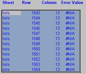
Locating errors in files
Here is the code I have recently developed to locate and report all the errors in a file.
To make this work I have created a sheet for the error list and named a range (single cell) on the sheet "cellerror_date". Two rows above that (with a blank row between) are the four headings, Sheet, Row, Column and Error Value.
Now add to a module in the Visual Basic Editor the follow statements.
Option Base 1
Dim LastRow&, LastCol%
Dim lastcellRowno, lastcellColno
Then add this function.
Function LastCell(ws As Worksheet) As Range
' Function written December 2004 by www.jethromanagement.biz
' Error-handling in case there is no data in the worksheet
On Error Resume Next
With ws
' Find the last real row
LastRow& = .Cells.Find(What:="*", SearchDirection:=xlPrevious, SearchOrder:=xlByRows).Row
' Find the last real column
LastCol% = .Cells.Find(What:="*", SearchDirection:=xlPrevious, SearchOrder:=xlByColumns).Column
End With
'initialize a Range object variable for the last populated row.
Set LastCell = ws.Cells(LastRow&, LastCol%)
End Function
Finally add this procedure.
Sub find_errors()
' Macro written December 2004 by www.jethromanagement.biz
Dim x, z
Dim c
Dim cellerrors()
Application.ScreenUpdating = False
'clear out last error check results
Application.Goto reference:="cellerror_data"
Selection.CurrentRegion.Select
Selection.ClearContents
'cycle once to count errors
x = 1
For Each ws In Sheets
ws.Activate
'identify the last cell
lastcellRowno = LastCell(ActiveSheet).Row
lastcellColno = LastCell(ActiveSheet).Column
'select range to the last cell in worksheet
Range("A1").Select
Range(ActiveCell, ActiveCell.Offset(lastcellRowno - 1, lastcellColno - 1)).Select
'check if any cells have errors
For Each c In Selection.Cells
If IsError(c) Then
x = x + 1 'count number of errors
End If
Next c
Next ws
'cycle again pasting errors to array
ReDim cellerrors(x, 4)
z = 1
For Each ws In Sheets
ws.Activate
'identify the last cell
lastcellRowno = LastCell(ActiveSheet).Row
lastcellColno = LastCell(ActiveSheet).Column
'select range to the last cell in worksheet
Range("A1").Select
Range(ActiveCell, ActiveCell.Offset(lastcellRowno - 1, lastcellColno - 1)).Select
'check if any cells have errors - then add error data to array
For Each c In Selection.Cells
If IsError(c) Then
cellerrors(z, 1) = ws.Name
cellerrors(z, 2) = c.Row
cellerrors(z, 3) = c.Column
cellerrors(z, 4) = c.Formula
z = z + 1
End If
Next c
Next ws
'paste array into error worksheet
Application.Goto reference:="cellerror_data"
Range(ActiveCell, ActiveCell.Offset(x - 2, 3)).Select
Selection = cellerrors
Application.ScreenUpdating = False
End Sub
Run the macro titled find_errors to locate all errors on any sheet in the book (including hidden sheets) and record their location and value.
Fractions versus Dates in Excel
Ian writes about the problem Excel has with determining 1/4 as either a date or a fraction.
By adding a zero to the front of the fraction Excel will know for certain that "0 1/4" should be a fraction instead of January 4th.
He also details the formatting requirements to make Excel format numbers that way you want.
For example when you change something like 4.235 to display as a fraction, "4 1/4" is displayed. Click Format | Cells | Number tab and then choose Fraction from the list of number formats. A list of fraction display choices will pop up, allowing you to change from the default of one fraction digit to two or three, turning 4.235 into "4 4/17" or "4 47/200," respectively.
Saturday, January 01, 2005
New Year and Dates in Excel
Happy New Year!
Don't forget that Excel automically does some date formatting for you.
Here's the basic rules to be wary of.
Note for the Amercians the dates are round the right way - you can swap the month and day to get it all backward the way you like it. (I think the answers are the same.)
When entering dates Excel will complete partly entered dates. Eg if you type 15/5 in a cell and hit Enter then you will get the 15th of May 2005 not 3. If you wanted 3 then type =15/5 and hit enter. (Not in the same cell or you will get 3-Jan (in the year 1900. You could reformat this however because it is the correct information, just not the correct format).
Notice that if you type 15/5 and hit Enter that it comes up 15-May. However if you click on the cell you will see in the formula bar that it is 15/05/2005.
So the first thing to be wary of is that Excel will automatically complete the year in a partly entered date (day and month) - using the current year.
If you wanted 15 May 2004 then you would need to either edit the year in that cell or type 15/5/04 and hit Enter.
The next thing to look at is the automatic year cutoff.
This is when you enter a year in the yy format. (It is better to use yyyy and then the following problem will never occur) For example enter 15/5/04 as above and you will get 15 May 2004. This time Excel is using a rule based on 1929. If you enter any date after (and including) 1 Jan 1930 and enter "30" as the year then you will get the date between now and 1930. If you enter a date year between 05 and 29 inclusive then it wil automatically assume that it is future and give you 2005-20029 as entered.
Test this by typing 15/5/29 in a cell and hitting Enter, then try 15/5/31.
The trick to be careful of is when working with dates from between 2005 and 2030 and on into the future. Enter the full year date for any year after or including 2030 or you will get 1930 instead wieh potnetially disstrous results for your spreadsheet.
The Excel Guru's Free Tips and Hints.

Welcome
Welcome to the Excel Tips blog. Free Microsoft Excel Tips and Hints designed to increase your productivity.
Advertisement
Subscribe Me
Previous Posts
- New Website
- New Open XML file formats in Office 2007
- Maximum Length of Macros
- Undiscovered Excel Funtions and Features
- Excel VBA Macro Shortcut Keys
- Excel 2007 Tips
- List of Macro Shortcuts in All Open Workbooks
- Excel 2003-2007 conversion project
- Excel 2007 and backward compatibility
- Clear Excess Formatting in Excel Files
My Blogs and Websites
- Spy Journal Home
- Spy Journal Archives
 Personal Blog
- Excel Tips Blog
- Blog Tips Blog
- Tech Tips Blog
- Urban Space Novel
- Photo Archive
- Parklife Results
- Parklife Soccer Club Website
- KROSTech LAN Parties
- Jethro Management
- Jethro Consultants
- Oz Bush Poet
Excel Links
- ---RSS Feeds---
- Unofficial Microsoft Office Stuff
- KC on Exchange and Outlook
- Office Zealot
- Automate Excel
- Colo's Excel Junk room
- Daily Dose Of Excel
- The Planning Deskbook
- Excel Pragma
- Andrew's Excel Tips
- ---No RSS Feed---
- Excel Tip
- Mailbarrow
- Experts Exchange
- AJP Excel Information
- Beyond Technology
- Contextures
- ExcelTip
- Mr Excel
- Pearson Software Consulting
- Peltier Technical Services
- John Walkenbach - J-Walk
- Vangelder (wont work in Firefox)
- VBA Express
- xlDynamic
- The Excel Nexus
- Code Net
- Better Solutions
- Excel Business Tools
- Data Pig Technologies
- VBA Express
Archives
- October 2004
- November 2004
- December 2004
- January 2005
- February 2005
- March 2005
- April 2005
- May 2005
- June 2005
- July 2005
- August 2005
- September 2005
- October 2005
- November 2005
- December 2005
- January 2006
- February 2006
- March 2006
- April 2006
- May 2006
- June 2006
- July 2006
- August 2006
- September 2006
- October 2006
- November 2006
- December 2006
- January 2007
- February 2007
- March 2007
- April 2007
- May 2007
- June 2007
- September 2007
- Current Posts
Other Links


Copyright Notice. All documents and text contained in this web site www.spyjournal.biz and sub pages is copyright material of Jethro Management (c) 2004 unless noted as being copyright material of someone else. No public reproduction of the content on this site in any form is permitted without express written permission.
Unless otherwise expressly stated, all original material of whatever nature created by Tim Miller and included in this weblog and any related pages, including the weblog's archives, is licensed under a Creative Commons License.