Spy Journal Excel Tips

Monday, November 29, 2004

Find text or values in Excel using VBA

This is some code that I use to locate specific text strings or values.

Note this code will not work as is, but will need you to complete the missing sections.
If you want to use this and don't know how to modify it yourself then email me back with your specific requirements and I can alter it for you.

Sub FindYourText()
Dim ts As Range
Set ts = ActiveSheet.Cells.Find(What:="your text string",Lookin:=xlValues)
If Not ts Is Nothing Then
'do whatever you need to do once you find it
End If
Set ts = Nothing
End Sub

Identifying the last cell in Excel

There are a number of ways to do this.

CTRL-END is the quickest way to locate the Last Cell in an Excel spreadsheet. Using F5 - Special - Last Cell is the actual command that CTRL + END performs.
This method does not always work because the used range (or "dirty area") of a spreadsheet may be larger than the area actually populated with your records.

Using VBA there are a number of methods as discussed below.
The Worksheet object's UsedRange does not always work for the same reason as the spreadsheet techniques described above.

The Range object's End method fails whenever you use the xlDown argument if it encounters a blank cell in the column being evaluated. However, if you use this same technique instead with the xlUp argument, starting from the bottom of the worksheet or just beneath the used range, it is almost bulletproof.
There may be memory issues related to this (associated with the real Last Cell).

Even so, there is a an even better way. The procedure below was written by Rodney Powell Microsoft MVP - Excel and adapted from a procedure written by MVP, Bob Umlas. They have tested it thoroughly and believe it's the most reliable way to accomplish this.

Function LastCell(ws As Worksheet) As Range
Dim LastRow&, LastCol%

' Error-handling is here in case there is not any
' data in the worksheet

On Error Resume Next

With ws

' Find the last real row

LastRow& = .Cells.Find(What:="*", _
SearchDirection:=xlPrevious, _
SearchOrder:=xlByRows).Row

' Find the last real column

LastCol% = .Cells.Find(What:="*", _
SearchDirection:=xlPrevious, _
SearchOrder:=xlByColumns).Column

End With

' Finally, initialize a Range object variable for
' the last populated row.

Set LastCell = ws.Cells(LastRow&, LastCol%)

End Function

Using this Function:

The LastCell function shown here would not be used in a worksheet, but would be called from another VBA procedure. Implementing it is as simple as the following example:

Sub Demo()

MsgBox LastCell(Sheet1).Row

End Sub

Thursday, November 25, 2004

VBA Macro in Excel for Finding Files in Folders

I use this base piece of code for finding files in the same subdirectory (or folder) that the file this code resides in is. I also use a modified version of it for known subdirectories.
The list of files gathered is processed in less than a second and can be pasted into the file or left in memory as an array and worked with. I use the latter process to open the files and work with them.

Paste the following code into a module in VBA Project Editor for Excel ensuring the that the top command, Option Base 1 is at the top of the module. The Dim statements can be made Public if desired.

Option Base 1
Sub find_files()
'Macro written by www.jethromanagement.biz September 2001
Dim thisfile, mydir, fname
Dim a, b
Dim flist()
Application.ScreenUpdating = False
'select subdir
'get filename and path
ThisWorkbook.Activate
fullfilename = ActiveWorkbook.FullName
'gets just the file name of this file
With ActiveWorkbook
thisfile = .Name
End With
'removes the filename to get the current drive and directory structure
mydir = Left(fullfilename, Len(fullfilename) - Len(thisfile))
'sets current drive to the drive in the path of the macro file
On Error GoTo nofiles
ChDir mydir
'find number of files
fname = mydir & "\*.xls"
a = 1
myname = Dir(fname) ' need to point it to the file mask
Do While myname <> "" ' Start the loop.
myname = Dir ' Get next filename
a = a + 1
Loop
'get file name data
ReDim flist(a - 1, 1)
b = 1
myname = Dir(fname) ' need to point it to the file mask
Do While myname <> "" ' Start the loop.
'extract file names during loop
Let flist(b, 1) = myname
myname = Dir ' Get next filename
b = b + 1
Loop
'enter file names into activecell - change to whatever range name you need
ActiveCell.Activate
Range(ActiveCell, ActiveCell.Offset(a - 2, 0)).Select
Selection = flist() 'fills selection with file names
Exit Sub
'error handler for no files
nofiles:
MsgBox "There were no files found."
nofiles = True
Application.ScreenUpdating = True
End Sub

Experts Exchange list Spy Journal Excel Tips

This site has been listed on the Experts Exchange website in the "Most Useful Microsoft Excel Resources on the Net" category.
Thats pretty nice.

Nicer would be some code to help those VBA users out there as requested today.
I will post it next.

Wednesday, November 24, 2004

Calculating Moving Averages in Excel

Reader's Request:

"How do I calculate a moving average in Excel?"

Moving averages are actually quite simple and can be done a number of ways.

Excel has a chart function allowing a moving average trendline to be added to a chart. Try it. Create a line or bar chart and then select a series, right click and select Add Trendline. A dialog box of alternative trendlines will pop up. Select Moving Average and click OK.
Figure 1.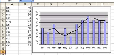

Moving Averages of Data

The following image illustrates two moving average calculations for some sales data.
First I created a table using the RAND() function. I then calulated two moving averages. The first is a simple formula of =AVERAGE(year1:year2) with the year totals being relative and not absolute . This formula is copied down and each calculation is for the year that the formula is on and the previous year
The second formula uses the relative $ on the row number to lock the starting year. Thus the range that the average is calculated over is progressivly larger as it is copied down. The last calculation is the average of all four years. This result gives an average that becomes less and less susceptible to movement as time goes on.

Your choice of method is dependent on the result you want to achieve.
The second method is good for predicting seasonality, the first is better for calculating margin variances between years.
Figure 2.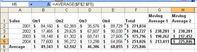

Tuesday, November 23, 2004

Using the formula bar in Excel

The formula bar is the blank line between the spreadsheet column headings and the toobars. It displays the formula of the currently selected cell.
It can be used in a number of ways.
Typing text into it or typing numbers.
Creating formulas using the function wizard fx or by typing them directly.
You can copy and paste into it and out of it.
You can debug or audit a formula by clicking the = button at the front of it. This allows you to view all the components of a function and where possible excel parses the formula compnents to provide individual results. You can also see these directly by clicking and selecting the part of the formula you want to resolve and hitting F9. This will resolve that part of the formula into a value. Be careful with this, if you then enter and save the change the formula will be overwritten with the value. However this is a useful way of quickly determining the value of part of a formula.

Monday, November 22, 2004

Using Format Painter in Excel, Word, Powerpoint and Publisher

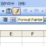
The format painter is a very useful tool. It appears in the Office applications, Word, Excel, Powerpoint and Publisher from 2000 on.
The simple method of using the painter is to select the text or cell that you want to copy the format from and then click the painter cicon on the tool bar. Wherever you click next, another cell or selection of text, you will "paint" the format. This can be a single cell or a selection of cells, or a selection of text.
This is an on and off function. Click on to paint and once you have painted it turns off.

You can paint multiple selections with the same format by double clicking the painter icon. Once you have done this everything you click on will get "painted" with the format until you release it by hitting escape.

You can paint multiple formats also. For example say you have a selection of 6 cells in Excel that have 6 different formats, eg in a table.
Select all 6 and then click the painter.
Now select six cells elsewhere and release the mouse button. They will all be painted with the relative formats. However if you select less cells in your target range than your source range the formats will only be pasted in as many as you select. Eg unselected cells will not be painted.

Note: The format painter will not paste column or row widths.

Make Excel Talk

Found on AutomateExcel.com
Excellent stuff!

Do you have a newer edition of Excel with "Text to Speech" installed? If so, you can make Excel speak from VBA code. Don't forget to turn up your speakers.

The following will speak the text in cell A1 of the ActiveSheet:

Sub SayThisCell()
Cells(1, 1).Speak
End Sub

This next Macro doesn't require text to be in any spreadsheet, it speaks the contents of a string:

Sub SayThisString()
Dim SayThis As String

SayThis = "I love Microsoft Excel"
Application.Speech.Speak (SayThis)

End Sub

Friday, November 19, 2004

Readers requests for tips

Do you have a specific question you would like answered?
Email me (using the link on the side bar) and I will publish the answer to your question on the website. No personal or confidential details will be published.

Thursday, November 18, 2004

Using the RAND function in Excel

Excel has lots of mathematical, trigonometrical and statistical functions (amongst many other categories)

One of the more obsucure ones is the =RAND() function. Using ths function in a cell simply returns a random number between 0 and 1. I have found my default setting in excel generates a number with 15 decimal places eg 0.621329327946131.
If you cannot see that many decimal places (excel defaults to 9) then expand the number of decimal places.

Here are some ways I use the RAND function.

Generating dummy data.
I combine RAND with the ROUND function to give me the level of precision I want.
=ROUND(RAND(),3)*1000 will return a result between 1 and 1000.
=ROUND(RAND()*1000000,-3) will return an even hundred thousand result between 100,000 and 1,000,000.

Generating random passwords.
First create two columns as follows. A1-A26 fill with numbers 1 to 36, B1-B36 fill with a to z and 0 to 9. Select all this data and name this range "alphanum"
Now copy the following formula into a cell.
=VLOOKUP(INT(ROUND(1+RAND()*37,0)),alphanum,2,TRUE)&VLOOKUP(INT(ROUND(1+RAND()*37,0)),alphanum,2,TRUE)
This will return a two character password. Adding additional elements of &VLOOKUP(INT(ROUND(1+RAND()*37,0)),alphanum,2,TRUE) to the formula will increase the number of characters.

Hiding and Unhiding rows and Columns in Excel

I have come across a keyboard short cut for hiding and unhiding rows and columns in Excel.
CTRL+9: Hide rows
CTRL+SHIFT+( (opening parenthesis): Unhide rows
CTRL+0 (zero): Hide columns
CTRL+SHIFT+) (closing parenthesis): Unhide columns

These are actually on my shortcuts page but I had never used them before.

Tuesday, November 16, 2004

Fun with Excel

I have some fun Excel stuff stored on my company website
These include Conways game of Life recreated in an Excel spreadsheet, A ticking analog clock in an Excel spreadsheet, short cuts for the VBA editor and playing with userforms.

Using the SUMIF Function in Excel

I use the SUMIF function a lot of the time, maybe too much if thats possible!

Basically the SUMIF funciton sums a range of data based on the criteria it finds in an adjacent range.

So if you have two columns A & B, A with names in it and B with weekly salaries, then you can use the SUMIF function to fnd the total paid to each individual payee.

=SUMIF($A:$A,"Fred",$B:$B)

Note. The criteria (in this case "Fred") must be spelt exactly the same way as in the lookup range (in this case column A). Otherwise it wont be added, this includes trailing spaces in cell contents.

Saturday, November 13, 2004

Using Logic Functions in Excel

The logical function =IF(logical_test,if_true,if_false) can be used in Excel to make a logical decision. If you want to perform more complex comparisions you can add the logical functions AND(), OR() and NOT() when you use the IF() function. Here are some examples on how to use these functions.

When using the IF function to perform a logical test, you can use one of the following compare methods:
= Equal to
<> Not equal to
> Greater than
>= Greater than or equal to
< Less than
<= Less than or equal to

Definitions of the logical functions in Excel.
AND() = TRUE if all logical tests returns TRUE
OR() = TRUE if one logical test returns TRUE
NOT() = TRUE if the logical test returns FALSE
ISERR() = TRUE if the cell value is an error value different from #N/A
ISERROR() = TRUE if the cell value is an error value
ISNONTEXT() = TRUE if the cell value not is a text
ISNA() = TRUE if the cell value equals the error value #N/A
ISLOGICAL() = TRUE if the cell value is a logical value
ISREF() = TRUE if the cell value is a cell reference
ISNUMBER() = TRUE if the cell value is a number
ISTEXT() = TRUE if the cell value is a text
ISBLANK() = TRUE if the cell is empty (blank cell)

=AND(logical1,logical2...) This function can perform up to 30 logical tests and returns TRUE if ALL of the logical tests returns TRUE. If one or more logical tests returns FALSE it returns FALSE.

=OR(logical1,logical2...) This function can perform up to 30 logical tests and returns TRUE if at least ONE of the logical test returns TRUE. If none of the logical tests returns TRUE it returns FALSE.

=NOT(logical) This function will reverse the result from another logical function, and is often used to make it easier to understand the logical function.

Examples of logical functions in Excel
=IF(A1>=10,"The value in A1 is larger than 10","Not larger than 10")
=IF(ISBLANK(A1),"A1 must be filled in!","OK")
=IF(ISTEXT(A1),"A1 must be filled in with a number!","")
=IF(AND(A1>10,B1>20,C1>30),"All values are greater than","One or more values is less than")
=IF(OR(A1>10;B1>20;C1>30);"One or more values is greater than";"All values are less than")
=IF(NOT(A1>100),"Less than 100","Greater than 100")

Friday, November 12, 2004

Creating blank lines in an Excel Chart

I regularly put together charts of Actuals Vs Budgets.
In most instances these charts will be referencing database sheets in some way, usually via a subsidiary chart data summary formula area.

Usually there will be 12 months of a budget which will generally display a value, but the formula for the actuals will only display a value for months where there is data, and will display a zero where there is not.

While this is not a problem with bar charts in Excel, line and area charts will display incorrectly. Months with actual data will show correctly then the line or area will take a big dive towards zero and continue to display as a zero.

My solutions to this problem is to edit my formula to return #N/A as a result. The chart will ignore this error and not show any result at all.

Here's how I do that using an IF function.

=IF(formularesult=0,#N/A,formularesult) where formula result is the existing formula to generate the actual data.

Thursday, November 11, 2004

When To Automate Excel

(Reprinted from AutomateExcel)

Note to Office Managers: If your employees print something out of Excel to type the printout back into Excel, and do this consistently, you might need to automate.

Even Broader Scope: If your employees print anything out of the computer, to type the printout back into Excel, and do this consistently, you might need to automate.

Automate Excel: To make a process in Excel operate by VBA code, in order to reduce the amount of work done by people, increase the accuracy of the work done, and reduce the time taken to do the work.I bet you're very intelligent and can guess the final decision comes down to cost/benefit analysis(cost to automate vs. cost of doing the same), however this example is some of that "low hanging fruit" when looking for areas of improvement, incredibly easy to identify, and also a classic and sometimes hilarious example of when to automate.

Email me for a quote if you have any upcoming automation projects.

Tuesday, November 09, 2004

Macro for Deleting Blank Rows in Excel

Following is a macro that will delete blank rows from a selected range in an excel sheet. It looks at a range of multiple rows and columns and only delete the rows that are completely blank. Great for use with imported data from an accounting package or similar that has blank rows in it.

Sub Delete_Blank_Rows()
'Deletes the entire row within the selection if the ENTIRE row contains no data.
'the Long type is used in case there is more than 32,767 rows in the selection

Dim x As Long

'Turn off calculation and screenupdating
With Application
.Calculation = xlCalculationManual
.ScreenUpdating = False

'work backwards because we are deleting rows and other wise the row number will change.
For x = Selection.Rows.Count To 1 Step -1
If WorksheetFunction.CountA(Selection.Rows(x)) = 0 Then
Selection.Rows(x).EntireRow.Delete
End If
Next x

.Calculation = xlCalculationAutomatic
.ScreenUpdating = True
End With
End Sub

If you want this customised to work with any particular spreadsheet you use then email me.

To use insert into a module in the VBA project editor (ALT + F11) and copy and paste the enitre italic above text in.

Saturday, November 06, 2004

Subtotal in Excel

A very useful function in Excel is the SUBTOTAL function. Using this in place of SUM in lists with subtotals in it allows for accurate summing of the entire list without having to link individual subtotals.

For example you may have a list of 10 values. The first 5 are subtotalled below in the same columm using the SUM function. The second 5 are also subtotalled using SUM. To get a grand total at the bottom you will need to add the two subtotal cells. (See the first image).
Using the SUBTOTAL function instead (option 9) will allow you to select the entire range and the command automatically ignores other subtotals. (See the second image)

A full list of the options available using the SUBTOTAL function can be found in the help. Reprinted here for your convenience.

Function_num(includes hidden values)
1 AVERAGE
2 COUNT
3 COUNTA
4 MAX
5 MIN
6 PRODUCT
7 STDEV
8 STDEVP
9 SUM
10 VAR
11 VARP

Function_num (ignores hidden values - only availble in Office 2003)
101 AVERAGE
102 COUNT
103 COUNTA
104 MAX
105 MIN
106 PRODUCT
107 STDEV
108 STDEVP
109 SUM
110 VAR
111 VARP

So using a function number in the SUBTOTAL function tells Excel to use that function in the formula result. Eg 4 will return the maximum value in the list.

Thursday, November 04, 2004

Summing two columns together in Excel

Have you ever needed to sum the results of two columns together. A common examplw would be a list of stock items and then quantity and unit cost.

Say you have the following three columns; A - Description, B - Quantity, C - Unit Cost.
Most people would create a fourth column for the value for each item being the Quantity times the Unit cost. They would then total this column for the total inventory value.

Well there are several other ways of doing it. (assume data in rows 2-11)

Use this normal formula =SUMPRODUCT(B2:B11,C2:C11)

Use an array formula (Press CTRL SHIFT ENTER when entering or editing the formula (CSE)) {=SUM(A2:A11*B2:B11)}
Note the {} come only after entering using CSE

Notes:
Both formulas will work across different sheets.
The CSE forumla will not work with a range of an entire row or column.

Wednesday, November 03, 2004

Sheet Shortcuts in Excel

Some great shortcuts to working with sheets in Excel.

Moving between sheets
CTRL + PGUP / PGDN

To find a particular sheet
Right click the sheet navigation arrows (at the far left of the sheet name tabs). This will bring up a list of all the sheet names. If there are more sheets then can fit in the list then a More Windows option will provide you with a dialog box to select from.

Copy sheets
Hold down CTRL, then drag a sheet tab right 1 sheet or left 2 sheets to copy it. A small plus will appear beside the mouse cursor indicating a new sheet will be created.

Rename sheet
Double click the sheet tab to edit the name.

Select multiple sheets
Hold down SHIFT whil using the CTRL +PGUP/PGDN shortcut.

Comprehensive list of Excel shortcuts

Tuesday, November 02, 2004

Add spaces to a string in Excel using REPT function

Thanks to Jon from PeltierTech for this one.

Generally when concatenating two text strings where I want a space between in Excel I use the formula:
= CONCATENATE(A1," ",B1)
If I wanted more than one space I would just add additional spaces to the formula.

Here is a better way.
= CONCATENATE(A1,REPT(" ",4),B1)
This formula will add 4 spaces to the string.

Monday, November 01, 2004

Excel Workbook Open Read Only Recommended

I had an email today from a client asking how to make a file read only for users. Here is my response.

Simply open the file, then click File - Save As and then in the dialog box click the Tools dropdown. From this select General Options. Check the Read-only recommended box and add a password to open and modify. If you make these two passwords different then you can hand out the password to open but not the password to modify. This way people are stuck with read only as the only option when opening the file. Note you will need to verify both the open and the modify password.

If you save over the existing file you will be asked to confirm that you want to overwrite the file.

VBA code to Unhide Sheets in Excel

I often hide sheets in Excel. This hides them from prying eyes (and fiddling fingers), and in the case of an Excel Workbook that is protected they are also unable to be unhidden.

Often however I will need to work on the hidden sheets. The manual process in Excel for this is to click Format - Sheet - Unhide from the menu. This will bring up a dialog box of the hidden sheets. You can select one sheet and unhide it. This becomes painful if you have a number of sheets to unhide.

Here is the code I use that will unhide them all rapidly.

Sub unhide_sheets()
'Macro written by Jethro Management
For Each ws In Sheets
ws.Visible = True
Next ws
End Sub

Simply copy and paste into an Excel VBA module and run it to unhide all sheets in an Excel Workbook.

Copyright Notice. All documents and text contained in this web site www.spyjournal.biz and sub pages is copyright material of Jethro Management (c) 2004 unless noted as being copyright material of someone else. No public reproduction of the content on this site in any form is permitted without express written permission.

Unless otherwise expressly stated, all original material of whatever nature created by Tim Miller and included in this weblog and any related pages, including the weblog's archives, is licensed under a Creative Commons License.

Monday, November 29, 2004

Thursday, November 25, 2004

Wednesday, November 24, 2004

Tuesday, November 23, 2004

Monday, November 22, 2004

Friday, November 19, 2004

Thursday, November 18, 2004

Tuesday, November 16, 2004

Saturday, November 13, 2004

Friday, November 12, 2004

Thursday, November 11, 2004

Tuesday, November 09, 2004

Saturday, November 06, 2004

Thursday, November 04, 2004

Wednesday, November 03, 2004

Tuesday, November 02, 2004

Monday, November 01, 2004

About Me

Welcome

Advertisement

Subscribe Me

Previous Posts

My Blogs and Websites

Excel Links

Archives

Other Links