Monday, February 27, 2006
SUMPRODUCT array formulas in Excel
I have written about these before as a way of summing data from tables using multiple selection criteria.
SUM(range) just sums a range of cells.
SUMIF(criteria range, criteria, sum range) sums data in one range based on results in a parallel range.
SUMPRODUCT((array1="criteria")*(array2="criteria")*(array3)) entered with CTRL SHIFT ENTER returns the sum of the data in the array3 where the crietria in arrays one and two are met. This can be expanded a lot.
Chris Pearson (as always) is one of the definitive sources for array forumlas.
Bob Phillips from the UK has written a very detailed page that very carefully explains how this works and how to use it with some practical examples.
Reading them both will give you some very valuable insights into how array formulas work and how to utilise them in your spreadsheets.
Some additional tips.
- Arrays must be the same dimensions.
- Having invalid information (eg text) in the array can be ignored using the double unary operator like so SUMPRODUCT(--(array1="criteria")*(array2="criteria")*(array3)).
- Arrays cannot be a whole column, but can be a whole row.
Finally, if anybody knows anything about how Office 12 will treat these types of formulas I am sure the Excel community would be interested to know.
Tuesday, February 21, 2006
Urgent Request
I am in urgent need of a top level Excel and VBA guru to work on a project for one of my clients for a couple of months - starting immediately.
If you can locate to Brisbane and be available for about 2 months we are prepared to pay a good rate.
Please contact me urgently if you are the person we need!
Tuesday, February 14, 2006
Resetting the last cell in Excel
Previously I have written about Identifying the last cell in Excel.
The microsoft website has an excellent article about how to reset the last cell.
Method 1
To reset the last cell by manually deleting excess rows and columns, follow these steps:
1. Select all columns to the right of the last column that contains data by selecting the appropriate column headings.
TIP: One way to do this is to press F5 and type the appropriate reference, for example F:IV for columns or 5:65536 for rows.
2. On the Edit menu, click Delete.
3. Repeat steps 1 and 2 for the rows that are under the last row that contains data.
4. On the File menu, click Save (click Save As if you want to keep the original file).
5. To continue working in the file, close, and then reopen the file.
Method 2
An Excel add-in to remove excess formatting and reset the last cell is now available for download. To download this add-in, visit the following Microsoft Web site:
Microsoft Downloads - excel addin
1. On the download page, click the Download button. When you are prompted to do so, click Open.
2. When you receive the licensing agreement, click Yes.
3. When you receive the WinZip Self-Extractor prompt, click the Browse button, and then select the location where you want the add-in to be extracted.
Note You can put the file in the Excel add-in location, where it will automatically show up in the Addins dialog box in Excel. That location is the Library folder in the Office install location, typically the C:\Program Files\Microsoft Office\Office\Library folder.
After you select the download location that you want in the Browse dialog box, click UnZip in the WinZip dialog box. Click OK on the successful download prompt, and then click Close in the WinZip dialog box.
4. Start Excel.
On the Tools menu, select Add-Ins. If you did not save the file to the Library folder, click the Browse button, locate the file, and then select it in the browse window. Click Excess Format Cleaner 1.1, and then click OK.
5. Open the workbook that you want to clean up, and then click Clear Excess Formatting in workbook on the File menu. The macro will then clear excess formatting from all worksheets in the file. When the macro is completed, you will be informed that you must save the workbook for the changes to be permanent.
6. Save, close, and then reopen the file.
Saturday, February 11, 2006
Using theTranspose function in Excel
Transposing in Excel refers to changing a range from vertical or horizontal orientation to the other.
One way to do this is to copy a range you want translated, eg a column of dates, and then using the Paste Special Function and selecting Transpose.
This will copy the exact range and translate it, but it doesn't allow you to create a dynamic range based on the previous range. In fact it works better if you select Paste As Values as well.
If you need to copy a columnar range and paste it as horizontal, yet have the target range change when the source range chanegs then the TRANSPOSE function is the way to do it.
Microsoft Excel Help says this about the TRANSPOSE function:
Returns a vertical range of cells as a horizontal range, or vice versa. TRANSPOSE must be entered as an array formula in a range that has the same number of rows and columns, respectively, as an array has columns and rows. Use TRANSPOSE to shift the vertical and horizontal orientation of an array on a worksheet.Note: The formula in the example must be entered as an array formula. To do this press CTRL+SHIFT+ENTER when entering the formula. If the formula is not entered as an array formula, the single result is 1.
Syntax
TRANSPOSE(array)
Array is an array or range of cells on a worksheet that you want to transpose. The transpose of an array is created by using the first row of the array as the first column of the new array, the second row of the array as the second column of the new array, and so on.
In my example we are going to copy a range of dates in a column and transpose them.
First of all enter your dates. I did this by typing =TODAY() in the first cell and then in the second cell added the cell above plus 1. This was then copied for 7 more cells giving 9 in total.
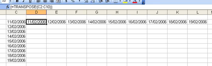
Now I select the cell I wanted the dates to go horizontally in. I also selected the 8 cells to the right, in total the same number of cells as the source array.
With them selected and the focus on the first cell I type =TRANSPOSE( and then select the 9 cells of dates in one column and finish up with the closing bracket. Now I hold down CTRL and SHIFT and click ENTER.
Presto! the 9 cells in the row now link directly to the dates in the column.
All that is needed is to format the cells to date format and we have our new horizontal date range linked to the vertical one. Change any of the vertical cells and the horizontal ones reflect the same change.
Tuesday, February 07, 2006
Excel MVP and Professional Guru association ideas
Interesting discussion on Dicks Blog regarding Excel MVPs.
Heres my two cents.
If I may add my two cents I think that the MVP program should remain firmly where it is (as defined by Sean) and that a separate peer nominated program for Guru status (technical competence) be created. It should be separate to Microsoft and probably be a professional organisation. It whould not be based on fee for service but be nominated by users clients or by yourself and then judged on a number of tecnhical merits.
As in any undertaking like this there would be numerous pitfalls to overcome in the first rounds of creation and ongoing tweaks to be made, but this could be recognised and dealt with by 5 yearly reviews of the system.
The concept of fellows within this organisation should definitely be promoted.
My pick for lifetime members is obiously biased by my reality but would definitely include John Walkenbach, Chip Pearson.
Founding members would include Dick, Jon, Steve, Andy, Colo and more (not trying to leave anybody out).
Professional membership fees would be charged to cover the admin costs of such a professional body.
What do you think?
The Excel Guru's Free Tips and Hints.

Welcome
Welcome to the Excel Tips blog. Free Microsoft Excel Tips and Hints designed to increase your productivity.
Advertisement
Subscribe Me
Previous Posts
- New Website
- New Open XML file formats in Office 2007
- Maximum Length of Macros
- Undiscovered Excel Funtions and Features
- Excel VBA Macro Shortcut Keys
- Excel 2007 Tips
- List of Macro Shortcuts in All Open Workbooks
- Excel 2003-2007 conversion project
- Excel 2007 and backward compatibility
- Clear Excess Formatting in Excel Files
My Blogs and Websites
- Spy Journal Home
- Spy Journal Archives
 Personal Blog
- Excel Tips Blog
- Blog Tips Blog
- Tech Tips Blog
- Urban Space Novel
- Photo Archive
- Parklife Results
- Parklife Soccer Club Website
- KROSTech LAN Parties
- Jethro Management
- Jethro Consultants
- Oz Bush Poet
Excel Links
- ---RSS Feeds---
- Unofficial Microsoft Office Stuff
- KC on Exchange and Outlook
- Office Zealot
- Automate Excel
- Colo's Excel Junk room
- Daily Dose Of Excel
- The Planning Deskbook
- Excel Pragma
- Andrew's Excel Tips
- ---No RSS Feed---
- Excel Tip
- Mailbarrow
- Experts Exchange
- AJP Excel Information
- Beyond Technology
- Contextures
- ExcelTip
- Mr Excel
- Pearson Software Consulting
- Peltier Technical Services
- John Walkenbach - J-Walk
- Vangelder (wont work in Firefox)
- VBA Express
- xlDynamic
- The Excel Nexus
- Code Net
- Better Solutions
- Excel Business Tools
- Data Pig Technologies
- VBA Express
Archives
- October 2004
- November 2004
- December 2004
- January 2005
- February 2005
- March 2005
- April 2005
- May 2005
- June 2005
- July 2005
- August 2005
- September 2005
- October 2005
- November 2005
- December 2005
- January 2006
- February 2006
- March 2006
- April 2006
- May 2006
- June 2006
- July 2006
- August 2006
- September 2006
- October 2006
- November 2006
- December 2006
- January 2007
- February 2007
- March 2007
- April 2007
- May 2007
- June 2007
- September 2007
- Current Posts
Other Links


Copyright Notice. All documents and text contained in this web site www.spyjournal.biz and sub pages is copyright material of Jethro Management (c) 2004 unless noted as being copyright material of someone else. No public reproduction of the content on this site in any form is permitted without express written permission.
Unless otherwise expressly stated, all original material of whatever nature created by Tim Miller and included in this weblog and any related pages, including the weblog's archives, is licensed under a Creative Commons License.