Monday, February 28, 2005
Another Excel Site
Just found another great Excel site.
Andrew is a self confessed Excel Fanatic!
He has some great resources on his web site. Check it out.
Sunday, February 27, 2005
AND and OR Functions in Excel
Logic functions in Excel follow the same rules you learnt at school (or didn't learn as the case maybe.
AND requries all the arguments of the function to return a TRUE result in order to return TRUE. If any 1 argument returns FALSE then the entire funciton will return FALSE.
OR on the other hand requires any 1 argument to return TRUE and the result will be TRUE regardless of how many FALSE arguments there may be.
If all that was gobbledy-gook then let me use some examples to illustrate how people use these logic structures everday without even noticing.
Your car battery is charged = TRUE, AND your fuel tank is not empty = TRUE makes you can start your car = TRUE. If either of these arguments returns a FALSE result then you cannot start your car and the function result is FALSE.
You are a male OR you are a female = TRUE. Regardless of the result of either individual argument, as long as one of them is TRUE (and I hope its is for you dear reader!) then the result is TRUE.
So how do we use this in Excel?
Typically I will use the AND statement to return a result where I need all the individual components to be TRUE before getting a correct answer.
Thus in a spreadsheet containing 3 columns of data I can check that each column has specific data in it by adding a 4th column to validate it.
EG =AND(A1<>"",B1<>"",C1<>"")
This checks cells A1, B1 and C1 to see if they contain something (anything except an empty cell will return TRUE for each argument). If any of the cells is blank then my validation formula will return FALSE.
I use AND in my article about conditional formatting.
OR I use to test results. Eg testing a cell where gender is required to be entered as either M or F. Here a formula such as =OR(A1="M",A1="F") can be used. If either of these values are entered then the formula will return TRUE. If nothing or an alternative gender is entered than FALSE is returned.
This is obviously just brushing the field of logic. Far more complex calculations can be created and used. Contact me if you think you can benefit from learning more about this.
Free XML Developers Book
Essential XML Quick Reference: A Programmer's Reference to XML, XPath, XSLT, XML Schema, SOAP, and More
Addison-Wesley and Developmentor have provided TheServerSide.NET with the entire book of Essential XML Quick Reference for free download. Essential XML Quick Reference is for anyone working with today's mainstream XML technologies. It was specifically designed to serve as a handy but thorough quick reference that answers the most common XML-related technical questions.It goes beyond the traditional pocket reference design by providing complete coverage of each topic along with plenty of meaningful examples. Each chapter provides a brief introduction, which is followed by the detailed reference information. This approach assumes the reader has a basic understanding of the given topic.The detailed outline (at the beginning), index (in the back), bleeding tabs (along the side), and the page headers/footers were designed to help readers quickly find answers to their questions.
Download the free PDF file from this website. (8.8Mb)
Thursday, February 24, 2005
Freezing Panes In Excel
Did you know you can freeze panes in Excel?
What this means is that you can set a portion of the screen either at the top, or the left or both that does not move as you scroll down or right.
Why would you do this?
If you have data in columns and you want to see the top header no matter how far down you scroll then select the cell in column a below the last row you want to "fix" in position. Use Windows | Freeze Panes to set the top rows.
If you have data at the left you want to see, eg a customer name while scrolling right to view columns of data then select the cell in row 1 one column to the right of the last column you want to "fix" in position. Use Windows | Freeze Panes to set the left columns.
Using any other location will fix all rows above and all columns left of the cell selected.
Tuesday, February 22, 2005
Edit Directly in Cell in Excel
Under the Tools | Options menu on the Edit tab there is a check box next to an item called Edit Directly in Cell.
By default this is turned on.
However turning it off allows access to a couple of cool features.
The first is editing in the function bar and not in the cell (as the name implies). This may not sound very cool, but when you have a long formula it pays off big time.
If you also have a formula that links to a lot of other cells or ranges on that same sheet, then these are all colour coded and easy to see when you first press F2 to edit the formula.
The second feature is not obvious at all. However turning off the option gives you the ability to double click a cell and be magically transported to the origin of that cell. Now this gets a little tricky with ranges or multiple selections, but is sure is a handy way to trace links back. Try it. On a sheet make a cell = to a cell on another sheet. Eg on Sheet1 put this formula in a cell. =+Sheet2!B29.
Now double click that cell. You will be taken to Sheet2, cell B29. This even works across open workbooks.
Saturday, February 19, 2005
Using text in Excel
One of my pet hates is people who use Excel as a wordprocessor. I often have to fix up problems caused by errant spaces left in cells.
However Excel does have some useful wordprocessing abilities that can come in handy. If I have to produce text together with graphs, tables of data etc then I prefer to use Excel than Word, even though Word has far superior desk top processsing abilities. If the data is not going to change I tend to copy and paste into Word but if it is to be dynamic than I don't like to link it live as its not hard for the links to go screwy.
In Excel you can wrap text in a cell, Merge cells together to make larger cells (be careful doing this), and align text vertically and horizontally. Use the Format Cells Alignment tab to do this.
You can also justify text within a range. Use Edit | Fill | Justify for this.
Spell check is also available - F7.
Friday, February 18, 2005
Using Expandable Range names in Excel
There are several ways to create range names in Excel and they have multiple uses. Here I talk about how to use them in a Data | Validation | List option.
I like to use the Validation List option to create drop down boxes for selections. I like to use range names for the lists for the selections.
I have discovered that if you create a range name fixed, Eg =$A$1:$A$5 for five selections, that if you want to add another option then you either have to insert a row (or cell) in the middle of the selection or change the range name. This is of course annoying (especially if you forget to change the range) and its not always possible to insert a cell if that would affect other tables.
Another solution is to make the entire column the range name eg =$A:$A. The main problem with this is in lists created using the Data Validation becasue they contain the entire columns of options. (Lots of blank options that a user could select.)
Many years ago one of my readers Mark developed the concept of using the OFFSET function to create an ever expandable range name.
Use this formula in the range name creation box.
=OFFSET(sheet_name!$A$2,0,0,COUNTA(sheet_name!$A:$A)-1)
This formula assumes there is a header row (if not remove the -1 at the end) and that there is no other data in the column other than the list options. It counts the number of items in the column and subtracts 1 for the header row. It then uses this number to create a range offset from the starting cell (which could be a range name or cell reference) in this case $A$2 (assuming A1 is the header).
If this has confused the heck out of you and you wonder why on earth go to all this trouble then you obviously haven't discovered the power of drop down selections and range names. Give it a try.
Email me if you need help making this work in your applications.
Wednesday, February 16, 2005
Formula Auditing in Excel
Excel has some great visual auditing tools. To find them right click a blank part of the toolbar area and turn the Formula Auditing toolbar on.
The first button does error checking. It will check errors in the sheet. When it encounters them it will offer a number of options to help resolve the error.
The next five are the main auditing tools. Two are for tracing formula precedents and two for tracing dependants and the fifth is clear all arrows. The remainder of the buttons I will discuss another time.
The trace arrows are very useful for seeing all the precendents or dependants of a cell. Basically precedents are all cells that add to a cell somehow and dependents are all cells that use a cell in their formulas some how. To use it click on a cell that has a formula relying on other cells and then click the Trace Precedents button. Blue arrows will emanate from the cell leading to the cells or ranges that it uses in its calculation. Each successive click will take you back another generation from all the cells that were located each time. Clicking the Remove Precedent Arrows button removes one generation of arrows for each click.
Beware - this can be very slow on old computers if there are a lot of numbers because of the high graphics requirements to draw all the arrows.
Trace Dependants and Remove Trace Dependents work exactly the same way and locate all cells dependent on the cell selected. The Remove All Arrows button does just that.
The picture below shows an example of this in action.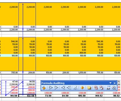
The blue lines generated are more than just pretty lines. They are also clickable. Double clicking them will send you along the line to the next cell. This is useful for cells that along way apart (off the screen). If your formula references another sheet then an arrow will head off left and up to a little black and white box representing an off sheet link. Double click the arrow leading to this box and you will open a box containing all the other sheet links that this arrow represented. Double clicking on any of these links will take you to that cell or range.
Tuesday, February 15, 2005
Sheet names in VBA code
Stino asked me about how to use the sheet name in VBA macro code after I posted about how to use sheet names in the file.
If your macro code has selected a cell or a sheet location then the name of the sheet can be located by using the Name object for the sheet thus Activesheet.Name.
If you are using code that is accessing the entire collection of worksheets (for example the password protection code I supplied previously) then the same object applies but the syntax is different.
To cycle through the sheets and use their names use this code.
For Each ws In Sheets
x= ws.Name
Next ws
Monday, February 14, 2005
More formatting tricks in Excel
I like to use a soft gray colour for borders around cells that need to be boxed. Eg a table.
First I turn the view gridlines off (Tools | Options).
Then I select the area to be boxed.
Then I use Format | Cells | Borders and select the grey colour, select the line weight and then click Inside and Outside.
After clicking OK I can then use the format painter to copy this selection anywhere else its needed.
Now I can use the black colour to create contrasting underlines where needed.
Example in the picture.
So how many of you picked the error in the PERMUT formula
Congratulations to Mark!
Tim,
PERMUT(4,2) is 12 not 24.
Mark
Saturday, February 12, 2005
Permutations and Combinations in Excel
These are two great functions in excel.
Combinations
The syntax is =COMBIN(Number, Number_chosen). The number is how many things you have. Eg 3 sandwich spreads. The number chosen is how many you want to combine. For example how many different combinations of 2 sandwich spreads can you make when you have 4 spreads available. The formula is =COMBIN(4,2) and the answer is 6 different combinations of two sandwich spreads.
A permutation is any set or subset of objects or events where internal order is significant. Permutations are different from combinations, for which the internal order is not significant.
So the number total number of permutations you can make from 4 objects using 2 objects.
from this formuls =PERMUT(4,2) and the answer is 12.
Thursday, February 10, 2005
Using Excel to make pretty pictures
No I was just kidding - I can't really do that. I am not real flash at art. But you can probably use the autoshapes and some of those fancy colours to do something artistic if you were so inclined.
Andrew from Automate Excel has a great article on how to create "see through" shapes. Create 3D effects for cubes etc and more.
Charles Maxson over at Office Zealot has an explanation of how to edit your colour selection palette to some real nice effects.
Brief summary of steps
1. Print Screen the source to duplicate
2. Paste the clipboard contents into Microsoft Paint
3. Use the Color Picker tool to select the color you want to use
4. From the Edit Colors dialog (Colors | Edit Colors…), click the Define Custom Colors… button to expand the dialog to revel the color settings
Click here to see what I am talking about...
Once you have the important RGB color settings from MS Paint, toggle over to Excel and create a routine similar to the following one where you apply your custom color’s RGB coordinates to alter the workbook’s Color properties. Note that your top-down RGB numbers from Paint go left-to-right in Excel:
Private Sub EditColor()
ActiveWorkbook.Colors(17) = RGB(255, 204, 0)
ActiveWorkbook.Colors(18) = RGB(255, 230, 130)
ActiveWorkbook.Colors(19) = RGB(153, 204, 0)
ActiveWorkbook.Colors(20) = RGB(236, 233, 216)
ActiveWorkbook.Colors(21) = RGB(255, 0, 0)
ActiveWorkbook.Colors(22) = RGB(0, 0, 153)
ActiveWorkbook.Colors(23) = RGB(255, 255, 153)
ActiveWorkbook.Colors(24) = RGB(71, 108, 145)
ActiveWorkbook.Colors(25) = RGB(0, 128, 0)
ActiveWorkbook.Colors(26) = RGB(255, 128, 0)
ActiveWorkbook.Colors(27) = RGB(33, 139, 254)
ActiveWorkbook.Colors(28) = RGB(217, 64, 64)
End Sub
Link for one of Charle's Excel samples in living color...
Tuesday, February 08, 2005
Working out a persons Age in Excel
Martin Green has written some very precise notes explaining the formula he has used to work out a persons age on any given day.
For all the details visit his website and review his explanation.
I will give you the formula and the explanation of each component.
=IF(MONTH(TODAY())>MONTH(A1),YEAR(TODAY())-YEAR(A1),
IF(AND(MONTH(TODAY())=MONTH(A1),DAY(TODAY())>=DAY(A1)),
YEAR(TODAY())-YEAR(A1),(YEAR(TODAY())-YEAR(A1))-1))
I've written this calculation on three lines for clarity but you should write is as a single expression without spaces. It assumes that cell A1 contains the person's date of birth. Here's what it says...IF(MONTH(TODAY())>MONTH(A1)
If this month is later than the month of the persons birthday...YEAR(TODAY())-YEAR(A1)
...subtract the year in which they were born from this year because they must have had their birthday.
But what if we haven't passed the month in which they were born. We might be in that month, or we might not have reached it yet. Let's find out...IF(AND(MONTH(TODAY())=MONTH(A1),DAY(TODAY())>=DAY(A1))
If we are currently in the month of the person's birthday and it is either their birthday today or we have passed it...YEAR(TODAY())-YEAR(A1)
...subtract the year in which they were born from this year because they must have had their birthday.
But what if this isn't the month in which they were born. We know we haven't passed their birthday so...(YEAR(TODAY())-YEAR(A1))-1
...subtract the year in which they were born from this year then subtract 1, because they haven't had their birthday yet.
Phew!
Sunday, February 06, 2005
Using the sheet name in an Excel file
Here is the formula I use in a file to get the sheet name.
=RIGHT(CELL("filename",A1),LEN(CELL("filename",A1)) -FIND("]",CELL("filename",A1)))
This always works because of the syntax that Excel uses in referencing.
Path[filename.xls]'sheet name'!cell reference
The '' marks around the sheet name only appear if the sheet name has certain special characters (eg space) in the name.
When ever you link a cell to another file the square brackets [] will always be around the file name.
When ever you link a to a cell on another sheet the sheet name and cell reference are always separated by the !.
The only exceptions are links to named ranges which can be on different sheets (and even different files. However the full syntax will be listed in the named range dialog box (CTRL F3).
Thursday, February 03, 2005
Using Conditional Formatting to flag due dates in Excel
I used the formulas in the image below to colour date cells in a column based on a age requirement. I needed to flag dates that were 4 years past the date entered Red as overdue, 1 month short of the 4 years Orange as a warning and 2 months short of 4 years Yellow so as to indicate the four years was almost up.
How I did it.
I selected one cell and went to the conditional formatting dialog box. (Format | Conditional Formatting).
Then I worked out the formula I needed. The AND formula requires that all events inside the brackets must be TRUE for the event to occur. In this case the date in the current cell plus 1461 days (4 years - including leap year) must be less than or equal to the current date TODAY() and the current cell must not be blank. In Excel <> is the way to express is not equal to.
I then added the second event and repeated the first formula but made it 1431 (less 30 days) plus the entered date to give a warning when 1 month away from 4 years.
Finally I added the third condition and used 1401 to be 60 days short of 4 years that the yellow warning will happen.
Note I have used relative formulas here. Once I completed it for one cell I copied that cell and then selected the entire column and Pasted Special as Formats.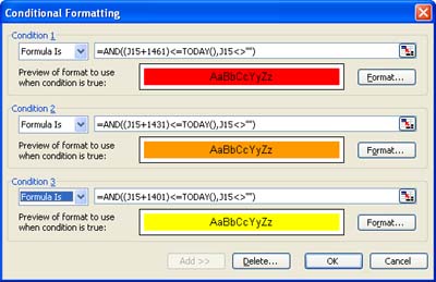
Wednesday, February 02, 2005
Double uses for buttons on Excel Toolbar
From Excel Tips
Some of the icons on the Standard and Formatting toolbars perform two different (but related) tasks. To toggle between the two tasks, press Shift while clicking the icon. The icons that perform different tasks are:
In the Standard toolbar:
*Print Print Preview
*Sort Ascending Sort Descending
*Open Save
*In the Formatting toolbar:
*Increase Indent Decrease Indent
*Underline Double Underline
*Center Merge and Center
*Increase Decimal Decrease Decimal
Example: The Open icon changed to Save when pressing the Shift key.
To remove the double-task icons:
Drag the icon off the toolbar while holding the Alt key.
The Excel Guru's Free Tips and Hints.

Welcome
Welcome to the Excel Tips blog. Free Microsoft Excel Tips and Hints designed to increase your productivity.
Advertisement
Subscribe Me
Previous Posts
- New Website
- New Open XML file formats in Office 2007
- Maximum Length of Macros
- Undiscovered Excel Funtions and Features
- Excel VBA Macro Shortcut Keys
- Excel 2007 Tips
- List of Macro Shortcuts in All Open Workbooks
- Excel 2003-2007 conversion project
- Excel 2007 and backward compatibility
- Clear Excess Formatting in Excel Files
My Blogs and Websites
- Spy Journal Home
- Spy Journal Archives
 Personal Blog
- Excel Tips Blog
- Blog Tips Blog
- Tech Tips Blog
- Urban Space Novel
- Photo Archive
- Parklife Results
- Parklife Soccer Club Website
- KROSTech LAN Parties
- Jethro Management
- Jethro Consultants
- Oz Bush Poet
Excel Links
- ---RSS Feeds---
- Unofficial Microsoft Office Stuff
- KC on Exchange and Outlook
- Office Zealot
- Automate Excel
- Colo's Excel Junk room
- Daily Dose Of Excel
- The Planning Deskbook
- Excel Pragma
- Andrew's Excel Tips
- ---No RSS Feed---
- Excel Tip
- Mailbarrow
- Experts Exchange
- AJP Excel Information
- Beyond Technology
- Contextures
- ExcelTip
- Mr Excel
- Pearson Software Consulting
- Peltier Technical Services
- John Walkenbach - J-Walk
- Vangelder (wont work in Firefox)
- VBA Express
- xlDynamic
- The Excel Nexus
- Code Net
- Better Solutions
- Excel Business Tools
- Data Pig Technologies
- VBA Express
Archives
- October 2004
- November 2004
- December 2004
- January 2005
- February 2005
- March 2005
- April 2005
- May 2005
- June 2005
- July 2005
- August 2005
- September 2005
- October 2005
- November 2005
- December 2005
- January 2006
- February 2006
- March 2006
- April 2006
- May 2006
- June 2006
- July 2006
- August 2006
- September 2006
- October 2006
- November 2006
- December 2006
- January 2007
- February 2007
- March 2007
- April 2007
- May 2007
- June 2007
- September 2007
- Current Posts
Other Links


Copyright Notice. All documents and text contained in this web site www.spyjournal.biz and sub pages is copyright material of Jethro Management (c) 2004 unless noted as being copyright material of someone else. No public reproduction of the content on this site in any form is permitted without express written permission.
Unless otherwise expressly stated, all original material of whatever nature created by Tim Miller and included in this weblog and any related pages, including the weblog's archives, is licensed under a Creative Commons License.