Thursday, February 03, 2005
Using Conditional Formatting to flag due dates in Excel
I used the formulas in the image below to colour date cells in a column based on a age requirement. I needed to flag dates that were 4 years past the date entered Red as overdue, 1 month short of the 4 years Orange as a warning and 2 months short of 4 years Yellow so as to indicate the four years was almost up.
How I did it.
I selected one cell and went to the conditional formatting dialog box. (Format | Conditional Formatting).
Then I worked out the formula I needed. The AND formula requires that all events inside the brackets must be TRUE for the event to occur. In this case the date in the current cell plus 1461 days (4 years - including leap year) must be less than or equal to the current date TODAY() and the current cell must not be blank. In Excel <> is the way to express is not equal to.
I then added the second event and repeated the first formula but made it 1431 (less 30 days) plus the entered date to give a warning when 1 month away from 4 years.
Finally I added the third condition and used 1401 to be 60 days short of 4 years that the yellow warning will happen.
Note I have used relative formulas here. Once I completed it for one cell I copied that cell and then selected the entire column and Pasted Special as Formats.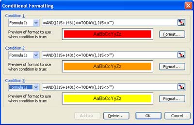
The Excel Guru's Free Tips and Hints.

Welcome
Welcome to the Excel Tips blog. Free Microsoft Excel Tips and Hints designed to increase your productivity.
Advertisement
Subscribe Me
Previous Posts
- Double uses for buttons on Excel Toolbar
- Protection in Excel Spreadsheets
- Changes to selecting all cells in Excel 2003 from ...
- New Zealand Excel Website
- Trick custom formats in Excel
- Arithmetic Operations in Excel
- Customise the toolbar in Excel
- SUMIF Formula in Excel
- CTRL SHIFT ENTER (CSE) Formulas in Excel
- Limiting the Movement in an Unprotected Sheet
My Blogs and Websites
- Spy Journal Home
- Spy Journal Archives
 Personal Blog
- Excel Tips Blog
- Blog Tips Blog
- Tech Tips Blog
- Urban Space Novel
- Photo Archive
- Parklife Results
- Parklife Soccer Club Website
- KROSTech LAN Parties
- Jethro Management
- Jethro Consultants
- Oz Bush Poet
Excel Links
- ---RSS Feeds---
- Unofficial Microsoft Office Stuff
- KC on Exchange and Outlook
- Office Zealot
- Automate Excel
- Colo's Excel Junk room
- Daily Dose Of Excel
- The Planning Deskbook
- Excel Pragma
- Andrew's Excel Tips
- ---No RSS Feed---
- Excel Tip
- Mailbarrow
- Experts Exchange
- AJP Excel Information
- Beyond Technology
- Contextures
- ExcelTip
- Mr Excel
- Pearson Software Consulting
- Peltier Technical Services
- John Walkenbach - J-Walk
- Vangelder (wont work in Firefox)
- VBA Express
- xlDynamic
- The Excel Nexus
- Code Net
- Better Solutions
- Excel Business Tools
- Data Pig Technologies
- VBA Express
Other Links


Copyright Notice. All documents and text contained in this web site www.spyjournal.biz and sub pages is copyright material of Jethro Management (c) 2004 unless noted as being copyright material of someone else. No public reproduction of the content on this site in any form is permitted without express written permission.
Unless otherwise expressly stated, all original material of whatever nature created by Tim Miller and included in this weblog and any related pages, including the weblog's archives, is licensed under a Creative Commons License.