Spy Journal Excel Tips

Saturday, October 30, 2004

Using the F5 Function key

Excel has a Goto function, and the shortcut is the F5 key.
Pressing this brings up a dialog box that allows you to select a named range or type in a cell reference, eg X95. This is useful if you want to select a cell in a hidden row or cell without having to unhide the row or cell. Clicking OK will take you to the required cell or range and make it active.

There is also a Special button. Clicking this brings up an advanced group of Goto options.

Some of the most useful ones include Blank Cells to select all the blank cells in an area and Formulas. Note if you want to select all the cells with a formula that results in an error then you can do this by selecting only the Errors option under Formulas.

Friday, October 29, 2004

Count the number of Unique Items in a Range

The following formulas are Array formulas. That means you need to press CTRL SHIFT ENTER when editing or entering the cell.

Use this formula to count the number of unique number items in a range.
=SUM(IF(FREQUENCY(A1:A10,A1:A10)>0,1))

Use this one to incoporate Text into the lookup.
=SUM(IF(FREQUENCY(MATCH(A1:A10,A1:A10,0),MATCH(A1:A10,A1:A10,0))>0,1))

Thursday, October 28, 2004

Creating Drop Down Lists Using Validation

You can create a drop down list easily in Excel by using the Validation command.

Validation allows you to apply preset parameters to a cell so that only certain entries can be made in the cell. For example you could limit it to dates between today and 7 days later.

In our example we are going to limit a cell to input from a predefined list using a drop down arrow.

First create a list of several items, eg Apple, Pear, Lemon, Orange.
Put each item in a separate cell, and these cells need to be next to each other either in 1 row or 1 column.

Select the cell in which the drop down list is to appear.
Click Data - Validation from the menu.
In the Settings Tab, choose List from the Allow box.
Click in the source box and click the red button at the end of it to minimise the dialog box then select the range with the list in it.
Click the red button again and then click OK.

You will now be able to use the drop down.

Advanced Options
Some more controls are available in the other tabs in the Validation box. Explore them to see how you can customise the drop down box.
You can copy validation from one cell to another using the Paste Special command.
You can use a range name in the source. Creating a range name for a specific range of cells restricts the drop down to only those cells.
Creating a dynamic range name or a range name that refers to an entire column or row will allow entry into the cell as well as drop down selection from the list. This is useful if the list is only a guide and not the only entries you want to allow.

Wednesday, October 27, 2004

Convert Text to Values and Values to Text

Converting text to values is easy using the VALUE function.
I generally insert a temporary column next to the column of text and create a formula =VALUE(A1) where A1 is the first cell in the range to change.
Fill the formula down.
Now select the formula range (eg Column B) and Copy then Paste Special as Values over the original cells.
Finally delete the temporary column.

Converting values back to text can be done a couple of ways.
For simple numbers in one cell you can use the CONCATENATE function but only concatenate the one cell. Eg =CONCATENATE(A1)
This however causes a problem if you want to maintain special formats, Eg Percents, Dates etc.
The way to convert these is to use the TEXT function.
Eg =TEXT(A1,"dd-mm-yyyy") will turn a date in cell a1 to text in the target cell with the format of dd-mm-yyyy. (For an explanatioin of date and time formats see this previous article)
The tip here is to use any valid format inside the quotes. You can determine the syntax of a valid format by looking inside the Format - Cells - Number - Custom dialog box.

Tuesday, October 26, 2004

Dynamic Range Names

If you have used a range name before then you will know that it can be frustrating updating the reference of the range name if you want to add data to the range.

Here are some ways you can dynamically update the range by using the OFFSET function in the range name reference.

Assume for all these examples that column A has a mixture of text and numbers for several cells.

Click Insert - Name - Define on the menu.
In the Names in Workbook Dialog box type a range name (Eg test_range) and then try these different options.

1: Expand Down as Many Rows as There are Numeric Entries.
In the Refers to box type: =OFFSET($A$1,0,0,COUNT($A:$A),1)

2: Expand Down as Many Rows as There are Numeric and Text Entries.
In the Refers to box type: =OFFSET($A$1,0,0,COUNTA($A:$A),1)

3: Expand Down to The Last Numeric Entry
In the Refers to box type: =OFFSET($A$1,0,0,MATCH(1E+306,$A:$A))
If you expect a number larger than 1E+306 (a one with 306 zeros) then change this to a larger number.

4: Expand Down to The Last Text Entry
In the Refers to box type: =OFFSET($A$1,0,0,MATCH("*",$A:$A,-1))

5: Expand Down Based on Another Cell Value
Put the number 10 in cell B1 first then:
In the Refers to box type: =OFFSET($A$1,0,0,$B$1,1)
Now change the number in cell B1 and the range will change accordingly.

6: Expand Down One Row Each Month
In the Refers to box type: =OFFSET($A$1,0,0,MONTH(TODAY()),1)

7: Expand Down One Row Each Week
In the Refers to box type: =OFFSET($A$1,0,0,WEEKNUM(TODAY()),1)
Requires the "Analysis Toolpak" to be installed. Tools>Add-ins-Analysis Toolpak

The good thing about number 3,4,5,6 and 7 is that they will include blank cells.

You can also change the Columns the dynamic range will span by simply changing the last Argument of the OFFSET function to a higher number than 1.
You could even expand across your Columns dynamically by placing another COUNT or COUNTA formula as the last argument, instead of 1. See below:

In the Refers to box type: =OFFSET($A$1,0,0,COUNTA($A:$A),COUNTA($1:$1))

This dynamic range will now also expand across Columns in Row 1. So if you add another Column to your Table the dynamic range will automatically incorporate it.

Adapted from OzGrid

Monday, October 25, 2004

XDate Extended Date Functions Add-In

Many users are surprised to discover that Excel cannot work with dates prior to the year 1900. The Extended Date Functions add-in (XDate) corrects this deficiency, and allows you to work with dates in the years 0100 through 9999.
John Walkenbach has the addin - download it for free.

Sunday, October 24, 2004

Protect and Unprotect Sheets Macro

I use some quick easy VBA code to protect and unprotect sheets. I will give you the two versions I use.

The first one is used where the password is obviously shown in the macro. The second "hides" the password. It doesn't really hide it but it is in a different spot and makes it less likely that users will find the password. Of course any users who really wanted to bypass the screen door protection of the Excel passwords would use the all internal passwords code I posted previously.

Simply copy and paste the text below into a module in the VBA editor.
You will need to ensure that all the sheets are either completely unlocked first or are all locked with the same password you use in the macro. This will work on hidden sheets also.

Visible password code
Copy this line into any module you like. Change the password in the quote marks to your required password.

Sub protect()
'protect macro
' Macro written by Jethro Management
Application.ScreenUpdating = False
For Each ws In Sheets
ws.protect Password:="expword"
Next ws
Application.ScreenUpdating = True
End Sub

Sub unprotect()
'unprotect macro
' Macro written by Jethro Management
Application.ScreenUpdating = False
For Each ws In Sheets
ws.unprotect Password:="expword"
Next ws
Application.ScreenUpdating = True
End Sub

Code with password stored as a Public Constant elsewhere

Copy this line into any module you like. Change the password in the quote marks to your required password.

Public Const expword As String = "expass"

The remainder of the code can go in any module also - doesnt have to be the same module that the password constant declaration is in.

Sub protect()
'protect macro
' Macro written by Jethro Management
Application.ScreenUpdating = False
For Each ws In Sheets
ws.protect Password:=expword
Next ws
Application.ScreenUpdating = True
End Sub

Sub unprotect()
'unprotect macro
' Macro written by Jethro Management
Application.ScreenUpdating = False
For Each ws In Sheets
ws.unprotect Password:=expword
Next ws
Application.ScreenUpdating = True
End Sub

If you need help then email me using the link on the right.

Friday, October 22, 2004

Excel Conditional Formatting Part 2

I know I said i would do this yesterday but I didn't. So sue me.

Following is a more advanced use of conditional formatting.

Alternate row shading.
Select all the cells you want to apply alternate row (or column) shading to
Select Format - Conditional Formatting from the menu.
Select Formula is from the Condition box.
In the formula box type =MOD(ROW(),2)=0 (or =MOD(COLUMN(),2)=0 for columns)
Click the format button and choose a pattern for the shading you want.
Click OK twice and shading will be applied.
To apply an alternate shading in the other row create a second condition by clicking the Add button.
Use this formula =MOD(ROW(),2)<>0 (or =MOD(COLUMN(),2)<>0 for columns)

How this works. The MOD function returns the remainder after dividing a number by an integer. Eg Divide 7 by 3 and the remainder is 1. In this case dividing the row number by 2 returns a remainder of 1 in an odd numbered row. So the first conditon will colour all even numbered rows. The second formula will colour all rows that return a remainder or odd numbered rows.

Wednesday, October 20, 2004

Using Excel to display text nicely

Sometimes you may need to have a fair amount of text in a cell or cells. Here are some tips to making that text look nice.

Justify
If you need to use several rows of cells to siplay a fair amount of text then you can use the Edit - Fill - Justify command to make this fit inside the cells.
To do this type all your text in the first cell.
Then select the range of cells you want the text to be spread over.
Select Edit - Fill - Justify and the text will flow down the range of cells and only fill as wide as the selection. Each cell in the first column will contain the text that fills to the width of the selection.
Note some fonts make this print differently to how it appears on the screen when multiple columns are being used.
If you need to edit cells and this changes the amount of text then re-performing the command with the selection will adjust it accordingly.
Note an error message will occur if the justified text will flow below the selected range, allowing you to back out if ncessary as it will other wise over write data in the cells below.

Alignment Wrap Text
You can also format a single cell or range of cells to wrap text within the cell. This row will then automatically adjust (or can be manually adjusted) to fit the depth of text entered.
Select the cell or cells, then Format - Cells select the Alignment tab and choose Wrap Text.
Using ALT + Enter gives you a carriage return or line feed between sentences if necessary.

Tuesday, October 19, 2004

Conditional Formatting in Excel

The conditional formatting feature of Excel has some pretty wide uses.

One of the main reasons I use it is for error checking.
It can be very useful to scan a large selection of data and look for a coloured cell out of place.

An example may be that you are processing a large selection of numbers in cells, and negative values need to be located or maybe you are looking for numbers over $1000 etc.
Select 1 cell in the range and choose Format - Conditional Formatting from the menu.

Use the first option Cell Value Is and then select the comparison phrase in the next drop down box, Eg less than. Now enter the value in the input box at the end. Eg 0. (In this example we will locate all cells where the value is less than 0 or a negative value.)
Now click the format button and select the pattern tab and choose red.
Click OK twice.
Now copy the cell and then select the entire range and Edit - Paste Special As - Formats.
All cells with negative values should now be coloured red. click on any of these cells and make the value positive and see the red disappear.

Tomorrow I shall discuss some more advanced uses of Conditional Formatting.

Excel Formula SUMPRODUCT

The SUMPRODUCT formula is a great way to calculate proportional totals.

The simplest way of using it is with an example of qty and value of stock items.

One way to find the total inventory value is by creating the last column that totals each individual row and is then summed. (Column D in the example below)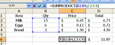

The alternative way is to create a SUMPRODUCT formula. The syntax is =SUMPRODUCT(range1, range2). See the formula in Cell C6 in the picture.
This adds the cumulative total of each row in the range multiplied by the second row. In this case that would return a result of $11.97. This would obviate the need for Column D.

SUMPRODUCT works both horizontally and vertically.

Sunday, October 17, 2004

Excel Paste Special Function

Most people know how to Copy and Paste in Excel. However few people know about the Paste Special function.

Open an excel spreadsheet and try these out. After selecting a cell select a target cell and then use Edit Paste Special to bring up the dialog box.

Paste
There are several different options available.
Formatting
Select Formats to only copy the cell formats from the source cell to the target cell. Note this includes conditional formatting.
Select Comments to only copy the cell comment from the source cell to the target cell.
Select Validation to only copy the cell validation options from the source cell to the target cell.
Select All Except Borders to copy the enitre cell content and formats except borders from the source cell to the target cell.
Select Column Widths to only copy the cell column width from the source cell to the target cell. This is especially useful if copying columns from one sheet to a blank new sheet. Paste Special the Column Widths first then paste the selection in normally afterwards.

Formulas
Select Formulas to only copy the cell formula from the source cell to the target cell. Note this does not change any formatting.
Select Formulas and Number Formats to only copy the cell formulas and number formats from the source cell to the target cell.

Values
Select Values to copy the cell contents as a value from the source cell to the target cell. This can be used to copy a selection that is derived by formula over itself so that it turns into values only. Useful if the original cell had a link to an external workbook that you want to break for example.
Select Values and Number Formats to copy the cell contents as a value and the number formats from the source cell to the target cell.

Operations
You can combine any of the Paste options with an Operation option but I won't discuss that here.
Arithmetic Functions
The simple use of these is to add, subtract, multiply or divide the target cell contents with the source cell contents.
For example copy a cell with a value of 3 and then Paste Special Add into a cell with a value of 4. It should change to a value of 7.
Copy a cell with 0 in it and Edit Paste Special Multiply onto a range of cells with formulas that return values to see that the formulas will be appended with *0 and the original formula will be inside brackets.

Transpose
This option enables you to switch a horizontal selection of cells into a vertical selection and vice versa. Be careful when doing this with cells with formulas linking other cells in them.

Links
Use this option to paste a range of cells into another range as a link back to the original range.

Saturday, October 16, 2004

Using the Excel Status bar for Quick Calculations

There is a cool feature in Excel on the status bar. Select any two or more cells that have values in them.
Now look down on the status bar just below the horizontal scroll bar. You should see the words "Sum=55" and the value will be the sum of the cells you selected.

This is a neat way of quickly checking the total of a group of cells. Non-adjacent cells can be selected using the CTRL key while clicking on cells.

Now right click the words "Sum=55" and a list of options will appear. These are None, Average, Count, Count Nums, Max, Min and Sum. Select any of these and that function will be performed on the selected cells and the result displayed in the status bar.

Note that the difference between Count and Count Nums is that Count will display the total number of non empty cells selected, while Count Nums will only display the total of cells selected with a value in them.

Friday, October 15, 2004

Office 12

The new version of Office - due probably around 2006 is called Office 12.
It may include an Excel server - though what this may do is as yet unclear.
Thanks to AutomateExcel for the news

Thursday, October 14, 2004

New Security Flaws in Excel

Thanks to AutomateExcel I picked up this news item from Secunia about the rash of security flaws MS has identified today along wth the required patches. I had already run 5 windows security patches on 7 machines today on my network. How many more are there?

Blog Tips site now available

My free blog tips site is now running. Here I (and some other contributors) will post short pithy explanations deisgned to help you understand the jargon of blogging, as well as "how to" articles. Check it out!

Wednesday, October 13, 2004

Using Pictures in Excel Charts Part 2

Nearly every part of an Excel Chart can have the area modified to a texture, a gradient fill, a pattern or a picture. What this means is that you don't have to use the standard Excel colours for the series of a chart, the background, the plot area, legend background etc.
Simple changes involve selecting a part of a chart, eg the chart area and using the format dialog to change it.
In the format dialog box choose the Patterns Tab. This is broken into two areas, Border and Area. At the bottom of the Area section is a button called Fill Effects. Clicking this opens another dialog box. This has 4 tabs, Gradient, Texture Pattern and Picture.
You can use the picture tab to select a picture from your pc or network and load it into the graph.
The other options are also useful. Patterns and textures can be used to create various effects. Gradient fills allow you to combine colours in groovy ways. There are even some Presets fills you can select.
As in all presentations, ensure you use contrasting and blending colours and fills and not garish combinations that set your viewers teeth on edge!

For a list of extensive advanced graph modifications including speedometer, thermometer, tile charts and other AJP Excel Information has some awesome examples and step by step instructions. Note these require a fairly advanced understanding of Excel Charts.

Tuesday, October 12, 2004

Formatting Dates and Times

There are some useful custom formats you can use when working with dates and times.

Dates
Select a cell with a date in it and then from the menu click Format - Cells and choose the Number Tab.
Select the Custom option.
The Type box on the right hand side is editable. Try these custom combinations.
d = Date in single digits Eg 8
dd = Date with two digits (leading zero for dates less than 10) Eg 08
ddd = Day of the week - short form 3 letter abbreviation Eg Fri
dddd = Day of the week - whole word Eg Friday
m = Month in single digits Eg 6
mm = Month with two digits (leading zero for dates less than 10) Eg 06
mmm = Month - short form 3 letter abbreviation Eg Jun
mmmm = Month - whole word Eg June
yy = Year in last two digits only Eg 04
yyyy = Year in full Eg 2004

Excel will allow you to use various separators including space, dashes, slashes etc. Experiment with what you want to see.

Time
Time is interesting. Negative time can be calculated but not displayed.
However there are some tricks to handling addition of time. It is all about understanding the bases. Time is managed in 4 parts. Seconds (base 60) Minutes (base 60) Hours (base 24) and AM/PM.
Type a time into a cell. The syntax to use is hh:mm:ss. You can shorten this by just typing the hour followed by the : to get the hour Eg 10: will give you 10:00:00 AM

However adding 10:00:00 to 15:00:00 will give you 1:00:00, because 10 hours plus 15 hours equals 25 hours which is 1AM. If you want to see 25:00 (for example in a timesheet spreadsheet) then format the cell custom to [h]:mm:ss
The bracketed h tells Excel to display the actual value and not parse it in base 24 format.

Monday, October 11, 2004

Using Pictures in Excel Charts Part 1

You can make charts look a little more visually appealing by using images in place of the normal columns.

Click on a series on a chart to select. Right-click and click Format Data Series. Add an image by choosing the Patterns tab and Fill Effects - Picture - Select Picture.
Once you've selected a picture, click on Insert and set the option for image scaling. The best options are Stack or Stack and Scale to. If you use the latter option, set the number of units that equal one image.
Don't worry if your picture looks "squished" in the Format Data Series dialog box, it will show up correctly in the chart.

There is a shortcut to the process that lets you use a clip-art image rather than an image from a file.
Select the data series and choose Insert - Picture - Clip Art. Once you've added the image, use the Fill Effects - Picture tab dialog to scale the clip-art image as you would if you had used an image from a file.

If the width of the column in the chart is too small for your image then you can alter it as folows.
Right-click on a series, choose Format Data Series - Options. Decrease the Gap Width to make the bars wider and if necessary add an overlap to widen the bars or columns even more.

Source PC MAgazine.

Saturday, October 09, 2004

Password Recovery Follow Up

I found the password recovery tool I was looking for but it had expired. Regnow can sell it to you for US$30 (US$60 for businesses).

Alternatively you can grab the free one I supplied the other day. All you need to do is copy and paste the VBA code into a module and run it.

Friday, October 08, 2004

Birthdays in Excel - TODAY and NOW

Did you know that all dates in Excel are handled as a serial number (starting 1 January 1900)?

Type in =TODAY() in a cell and then format the cell to General or Comma format.
When I did this (8th October 2004) I got 38268.

Now type your birthdate into another cell (using dd/mm/yyyy or mm/dd/yyyy format).
Once again you can format this with General or Comma to see the serial number associated with your birthdate.
You can now subtract your birthdate from today's date and see how many days you have been alive for - Scary huh!

The TODAY() function updates automatically whenever the spreadsheet is recalculated.

Now type =NOW() in another cell. This will give you the serial number associated with the hour, minute and second of the time right now. You may need to increase the number of decimal places showing to get this. This is represented by the part of a whole day (1) that is the correct time. For example midday equals 12:00:00 which translates to 0.5 or half a day.
Note that when you format the cell with =NOW() in it to General or Comma that it shows the serial number for today as the whole number to the left of the decimal point and the part of the day to this second as decimal places to the right.
Eg 38268.9965 is 11:55 PM on the 8th October. Happy Birthday to me!

The TODAY() function updates automatically whenever the spreadsheet is recalculated.

Conditional Formatting in Excel

Conditional formatting allows you to change the format of a cell depending on some criteria. These can be related to the cell itself or to some other cell on the same sheet.

An easy one to set up to see how this concept works is working with a list of $ values that have some negative values that you want to show in red.
You can use Conditional Formatting to check if the value of the cell is less than 0. If it is then make the font red. Try this out.

Select the range of data and then from the Format Menu choose Conditional Formatting.
In the dialog box make the following selections:
"Cell Value is"
"Less than"
"0" (just type a zero)
Then click Format and choose red in the font tab colour drop down box.
Click OK all the way out.

Negative values should now be displayed in Red. Note: conditional formatting has priority over any other formatting applied to a cell.

For a great article from Tip of the Day on How to shade Every Other Row in Excel using Conditional Formatting follow the link.

Thursday, October 07, 2004

Updates and Changes To Excel Tips

The feedback received so far has all been positive.
There will be some minor changes to the site as we tweak things.
I have created a mailing list of the posts for people who can't use the XML link to syndicate the site.
Because of Anti Spam legislation here in Australia I need you to email me if you want to be put on this list. Click the subscribe to email link on the right under my photo.
You can opt out from this mail out by replying and requesting to be removed at any time.
Thanks for reading.

Wednesday, October 06, 2004

Unprotecting Password Protected Sheets without the Password

Funny thing happened to day. I am halfway through reading this page from the Office Zealot about recovering pasword protected sheets when the phone rang. It is one of my tech guys wanting to know if I still had a password recovery tool. I said funny you should ask..

After a bit more of a read I decided to pass these two sites to you for your own use - they both supply a VBA macro that will unlock sheets where you have forgotten the password. Of course you would never use it to open someone else's file would you...

I have copied the All Internal Passwords code from McGimpsey into a text file here. Alternatively you can download a workbook with it inside from their site.

DISCLAIMER: Please note that breaking password protection MAY violate laws or regulations in your jurisdiction. If in doubt, ask the original author, and if you can't ask - don't use it!

Upgrade to Excel 2003

I bought Office 2003 Professional yesterday. Question was is the upgrade to Excel 2003 going to cause me the same amount of grief that the upgrade from Office 2000 to 2002(XP) did?
I still cannot listen to Vivaldi's Four Seasons without remembering the day and a half I spent listening to it on endless loop while on hold to Microsoft engineers the last time round. The only benefit was that the calls were free because I found real undocumented problems with the upgrade from 2000 to 2002(XP). If you are contemplating that upgrade then definitely email me so I can talk you through some of the issues you will potentially face. I may post some of them here later on.

Back to the current upgrade. I did some research online and found little actual reference to the upgrade in relation to Excel. Seems to be a non event.
However backward compatiability is important. I have some clients still using Excel 97.
About.com had an extensive review.

Microsoft pages
Sharepoint
Deployment
Upgrading Reference Page including links to the Office Converter Pack
Smart Documents (XML) Whitepaper
MS Excel 2003 Overview

For the techies. It would seem that the main reason for the upgrade is to support Microsoft's shift to the .NET framework. In particular the IRM and XML standards. However the XML features for both Word and Excel seems to be lacking in substance and XML schema tools at this point. As I have clients requiring XML export from Excel this is an interesting one for me.

I will post more information later on if I experience issues with the upgrade.

Reversing firstnames and surnames in a list

Today I wrote this formula for a friend who needed to convert a database field displaying names as surname firstname to firstname surname.
His data had been checked to see that only one space existed between each name in the list.
The formula written here was designed to provide the answer in Column B for the data in Column A.
=CONCATENATE(RIGHT(A1,LEN(A1)-FIND(" ",A1))," ",LEFT(A1,(FIND(" ",A1)-1)))
Once the formula had been filled down I instructed him to Copy it and then Paste Special As Values in the same place.
(More details on the Paste Special function tomorrow)

Tuesday, October 05, 2004

Using a slider to change a cell and a chart

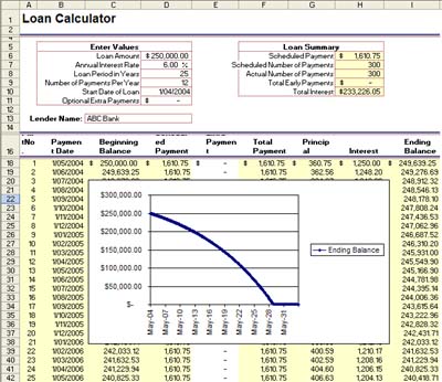
This is a cool function that can assist you to make easy to use adjustable tables.
Using the example of a mortgage, I used the loan wizard in Excel (under New Worksheet) to create a mortgage example. (Download Sample File). I then added a graph of the closing balance.
So now we have a nice looking chart that shows the closing balance of our mortgage over time.
Lets say we want to add the ability to easily change the additional payments and see graphically what that will do to our loan timeline.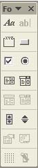

From the Forms toolbar select the scroll bar. Then drag your mouse over where you want it on your sheet while depressing the left button.
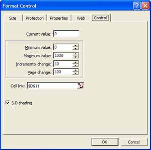
Now right click the control and select format control. Set it up as follows.
Now you can scroll up and down and as you do the additional payments changes by $10 a time, and the loan balance jumps accordingly. Clicking in the slider will cause it to page up or page down at $100 a time. Obviously you can make these settings what ever you desire for any application where you need to rapidly change 1 (or more) variable and see the results.

Monday, October 04, 2004

Quickly change Chart Titles in Excel

HAve you ever buit a bunch of charts from some data and presented them to your boss or client only for them to want the titles all changed? Maybe you want your chart titles to update with the date or month that the data is being presented for.

A quick way of doing this is to use links in the titles and not type the title into the chart options dialog box.

The quickest way I have found to do this is to actually type a couple of letters into the chart title in the Chart Options dialog Box and hit OK. This gives you a chart title that you can see and select. Once selected click in the formula bar, type = and then click the cell that has the chart title you want.
The chart title is instantly updated to the cell value. Note the cell can be a formula giving you a combination of text and values (eg using the formula CONCATENATE).

Changing the cell value automatically now changes the chart title. Link all your charts with the same name to the cell and "voila" - instant changes of chart titles when the cell link is changed.

Short Cut Keys in Excel save you time

Short cuts enable you to do stuff with Excel much faster. Typically these involve the keyboards as that is a faster way of operating than using a mouse.
Here are some of my most frequently used.

CTRL SHIFT and arrow keys - select cells (Hint: use the END key before an arrow to select blocks of cells)
CTRL SPACE - select a whole column
SHIFT SPACE - select a whole row
CTRL HOME - goes to the top left cell in the pane
CTRL + inserts a cell (or a row or column if the whole row or column is selected)
CTRL - deletes a cell (or a row or column if the whole row or column is selected)
CTRL PAGEUP - cycles up through the sheet tabs
CTRL PAGEDOWN - cycles down through the sheet tabs
CTRL D - fill down
CTRL R - fill right
CTRL INSERT - copy
SHIFT INSERT - paste
SHIFT DELETE - cut
F2 - edit formula
ALT F11 - open visual basic explorer
CTRL TAB or CTRL SHIFT TAB - cycles through open workbooks in forward and reverse

Comprehensive list of keyboard shortcuts

Welcome

Subscribe to this site using the RSS link to get free regular Microsoft Excel hints and tips.
Become more productive and create snappier spreadsheets.

Copyright Notice. All documents and text contained in this web site www.spyjournal.biz and sub pages is copyright material of Jethro Management (c) 2004 unless noted as being copyright material of someone else. No public reproduction of the content on this site in any form is permitted without express written permission.

Unless otherwise expressly stated, all original material of whatever nature created by Tim Miller and included in this weblog and any related pages, including the weblog's archives, is licensed under a Creative Commons License.