Friday, November 25, 2005
Using the Decimal Place Icons in Excel
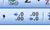 On the formatting toolbar in Excel are two buttons that work together.
These are the Increase and Decrease Decimal buttons.
You can use these to very quickly change the display of data. They work well in combination with the three standard format buttons before them on the toolbar, $(dollar) %(percent) and ,(comma). These format cells respectively as Currency (with two decimal places, Percent with no decimal places and comma seperated thousands with 2 decimal places.
If you want a different number of decimal places to be displayed then simply click either the increase or decrease decimal buttons to change the format of the selected cells.
Warning: Remember that the underlying data does not change. So changing Currency formatted data with two decimal places to no decimal places has no effect on the underlying data. Adding this data may give a different value to that when adding the face value (displayed) of the data. This is particularly important when printing reports. Although the data in a summed total may add accurately someone who picks up the printout may add the individual figures and sum them to a different result because they have no appreciation of the underlying decimal places.
Wednesday, November 16, 2005
Letting Go The Mouse - [2] Using the END key to select blocks
In the first post of this series I talked about how to use the SHIFT key with the arrow keys as an alternative to holding down the left mouse button and dragging to select cells.
Today I want to show you how to use the END key as a means to making that work a lot faster.
The END key is a toggle. Click it once and its on, click again and its off. It is easy to see which mode its in (on or off) in Excel because the status bar has an indicator next to the CAPS, NUM and SCRL indicators (bottom right corner).
Note the END key will not work as a toggle if the SCROLL LOCK is on so make sure it is off.
The END key allows you to quickly navigate through blocks of cells that are either empty (blank) or full (have data in them).
Lets assume we have a spreadsheet that has data in every cell in rows 1 through 5 and from column A to column Z and then blank cells through to column AZ then from column BA to BZ it is filled with data again.
If we are in Cell A1 and we want to select the data in the first block (A1:Z5) then we could use F5 and special and select the current region. But it is easier to hold down the SHIFT key, tap the END key and then tap the right arrow. This will select cells A1:Z1. Keep the SHIFT key depressed and tap the END key and the down arrow key. You should end up with the cells A1:Z5 selected. A grand total of 5 keystrokes.
Ok deselect by clicking on Cell A1 again (or using CTRL HOME).
Now lets see the easy way to select the cells BZ1:BZ5.
From cell A1 we know that there is a contiguous line of cells out to column Z then blank to column BA which has data in it.
Simply tap END then the right arrow key (no SHIFT this time). You should end up on Z1. Now do it again- tap END and right arrow. You should end up on Cell BA1. Notice that each time you hit something else when the END key is turned on it turns it off again.
To select this block do the same as for the first block.
Hold down the SHIFT key, tap the END key and then tap the right arrow. This will select cells BA1:BZ1. Keep the SHIFT key depressed and tap the END key and the down arrow key. You should end up with the cells BA1:BZ5 selected.
The END key becomes a powerful modifier to moving around a spreadsheet using the keyboard arrows. It soon becomes much quicker to use the keyboard to navigate around a spreadsheet then to use the mouse to scroll.
Tuesday, November 08, 2005
Letting Go the Mouse - [1] Using the SHIFT key to select cells in Excel
I have written here numerous times about keyboard shortcuts. There are so many and as you get to know then they become a lot quicker than using the mouse. However there are so many that it can be quite daunting looking at a list like this one http://www.jethromanagement.biz/ex_cuts.htm and knowing which ones will save you time and which ones won't.
This article is the first in a series entitled Letting Go the Mouse and is a guide to letting go the mouse and starting to use the keyboard.
The first thing I teach a mouse user who is oh-so-slow at using Excel is to use the keyboard to select cells.
How many times have you seen someone (or done it yourself) trying to select some data off the edge of the screen only to end up selecting 14000 rows or 85 columns because it scrolled too fast? Scrolling back up they take forever to get to the spot they wanted and usually go straight past and repeat this several times. It is frustrating for the person doing it and painful to watch.
LET GO THE MOUSE!
Use the keyboard for this. OK I will let you use the mouse to locate and select the top left cell of the selection. Of course you could select any corner of the selection but lets start with the most obvious, the top left cell.
Lets say we want to select 3 columns and 8 rows.
The key to this selection process is the SHIFT key. SHIFT allows you select a range of contiguous cells. That is cells that are adjacent to each other.
Experiment while holding the SHIFT key down with all the arrow keys one after the other.
Next time I will talk about selecting entire data or blank ranges.
The Excel Guru's Free Tips and Hints.

Welcome
Welcome to the Excel Tips blog. Free Microsoft Excel Tips and Hints designed to increase your productivity.
Advertisement
Subscribe Me
Previous Posts
- New Website
- New Open XML file formats in Office 2007
- Maximum Length of Macros
- Undiscovered Excel Funtions and Features
- Excel VBA Macro Shortcut Keys
- Excel 2007 Tips
- List of Macro Shortcuts in All Open Workbooks
- Excel 2003-2007 conversion project
- Excel 2007 and backward compatibility
- Clear Excess Formatting in Excel Files
My Blogs and Websites
- Spy Journal Home
- Spy Journal Archives
 Personal Blog
- Excel Tips Blog
- Blog Tips Blog
- Tech Tips Blog
- Urban Space Novel
- Photo Archive
- Parklife Results
- Parklife Soccer Club Website
- KROSTech LAN Parties
- Jethro Management
- Jethro Consultants
- Oz Bush Poet
Excel Links
- ---RSS Feeds---
- Unofficial Microsoft Office Stuff
- KC on Exchange and Outlook
- Office Zealot
- Automate Excel
- Colo's Excel Junk room
- Daily Dose Of Excel
- The Planning Deskbook
- Excel Pragma
- Andrew's Excel Tips
- ---No RSS Feed---
- Excel Tip
- Mailbarrow
- Experts Exchange
- AJP Excel Information
- Beyond Technology
- Contextures
- ExcelTip
- Mr Excel
- Pearson Software Consulting
- Peltier Technical Services
- John Walkenbach - J-Walk
- Vangelder (wont work in Firefox)
- VBA Express
- xlDynamic
- The Excel Nexus
- Code Net
- Better Solutions
- Excel Business Tools
- Data Pig Technologies
- VBA Express
Archives
- October 2004
- November 2004
- December 2004
- January 2005
- February 2005
- March 2005
- April 2005
- May 2005
- June 2005
- July 2005
- August 2005
- September 2005
- October 2005
- November 2005
- December 2005
- January 2006
- February 2006
- March 2006
- April 2006
- May 2006
- June 2006
- July 2006
- August 2006
- September 2006
- October 2006
- November 2006
- December 2006
- January 2007
- February 2007
- March 2007
- April 2007
- May 2007
- June 2007
- September 2007
- Current Posts
Other Links


Copyright Notice. All documents and text contained in this web site www.spyjournal.biz and sub pages is copyright material of Jethro Management (c) 2004 unless noted as being copyright material of someone else. No public reproduction of the content on this site in any form is permitted without express written permission.
Unless otherwise expressly stated, all original material of whatever nature created by Tim Miller and included in this weblog and any related pages, including the weblog's archives, is licensed under a Creative Commons License.