Saturday, February 11, 2006
Using theTranspose function in Excel
Transposing in Excel refers to changing a range from vertical or horizontal orientation to the other.
One way to do this is to copy a range you want translated, eg a column of dates, and then using the Paste Special Function and selecting Transpose.
This will copy the exact range and translate it, but it doesn't allow you to create a dynamic range based on the previous range. In fact it works better if you select Paste As Values as well.
If you need to copy a columnar range and paste it as horizontal, yet have the target range change when the source range chanegs then the TRANSPOSE function is the way to do it.
Microsoft Excel Help says this about the TRANSPOSE function:
Returns a vertical range of cells as a horizontal range, or vice versa. TRANSPOSE must be entered as an array formula in a range that has the same number of rows and columns, respectively, as an array has columns and rows. Use TRANSPOSE to shift the vertical and horizontal orientation of an array on a worksheet.Note: The formula in the example must be entered as an array formula. To do this press CTRL+SHIFT+ENTER when entering the formula. If the formula is not entered as an array formula, the single result is 1.
Syntax
TRANSPOSE(array)
Array is an array or range of cells on a worksheet that you want to transpose. The transpose of an array is created by using the first row of the array as the first column of the new array, the second row of the array as the second column of the new array, and so on.
In my example we are going to copy a range of dates in a column and transpose them.
First of all enter your dates. I did this by typing =TODAY() in the first cell and then in the second cell added the cell above plus 1. This was then copied for 7 more cells giving 9 in total.
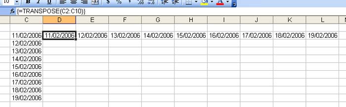
Now I select the cell I wanted the dates to go horizontally in. I also selected the 8 cells to the right, in total the same number of cells as the source array.
With them selected and the focus on the first cell I type =TRANSPOSE( and then select the 9 cells of dates in one column and finish up with the closing bracket. Now I hold down CTRL and SHIFT and click ENTER.
Presto! the 9 cells in the row now link directly to the dates in the column.
All that is needed is to format the cells to date format and we have our new horizontal date range linked to the vertical one. Change any of the vertical cells and the horizontal ones reflect the same change.
The Excel Guru's Free Tips and Hints.

Welcome
Welcome to the Excel Tips blog. Free Microsoft Excel Tips and Hints designed to increase your productivity.
Advertisement
Subscribe Me
Previous Posts
- Excel MVP and Professional Guru association ideas
- Debugging VBA
- De-Lurking Week
- Zooming an Excel spreadsheet for named ranges
- Reading complex formulas in Excel
- CTRL SHIFT ENTER Formulas in Excel
- Using the CTRL Key
- Speeding up Excel
- Tips for Printing in Excel
- Using the Decimal Place Icons in Excel
My Blogs and Websites
- Spy Journal Home
- Spy Journal Archives
 Personal Blog
- Excel Tips Blog
- Blog Tips Blog
- Tech Tips Blog
- Urban Space Novel
- Photo Archive
- Parklife Results
- Parklife Soccer Club Website
- KROSTech LAN Parties
- Jethro Management
- Jethro Consultants
- Oz Bush Poet
Excel Links
- ---RSS Feeds---
- Unofficial Microsoft Office Stuff
- KC on Exchange and Outlook
- Office Zealot
- Automate Excel
- Colo's Excel Junk room
- Daily Dose Of Excel
- The Planning Deskbook
- Excel Pragma
- Andrew's Excel Tips
- ---No RSS Feed---
- Excel Tip
- Mailbarrow
- Experts Exchange
- AJP Excel Information
- Beyond Technology
- Contextures
- ExcelTip
- Mr Excel
- Pearson Software Consulting
- Peltier Technical Services
- John Walkenbach - J-Walk
- Vangelder (wont work in Firefox)
- VBA Express
- xlDynamic
- The Excel Nexus
- Code Net
- Better Solutions
- Excel Business Tools
- Data Pig Technologies
- VBA Express
Other Links


Copyright Notice. All documents and text contained in this web site www.spyjournal.biz and sub pages is copyright material of Jethro Management (c) 2004 unless noted as being copyright material of someone else. No public reproduction of the content on this site in any form is permitted without express written permission.
Unless otherwise expressly stated, all original material of whatever nature created by Tim Miller and included in this weblog and any related pages, including the weblog's archives, is licensed under a Creative Commons License.