Excel
Excel Function of the Week - VLOOKUP & HLOOKUP
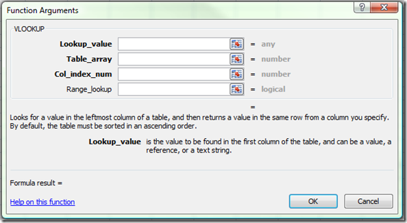
Mon, 15/12/2008 - 7:39pm — jethroI realised that when I wrote the ISNA function article that I had never written an explanation of VLOOKUP. I want to write up explanations for a umber of other functions in the future like COLUMN, ROW, MATCH and INDEX followed by OFFSET. All these make lots of sense when you use them with the VLOOKUP function. So I though it best to start with this function. I will also say that everything I write about VLOOKUP here applies to HLOOKUP as well. the only difference is the orientation, that is VLOOKUP looks across columns from left to right, and HLOOKUP looks down rows from top to bottom.
The built in Excel Help is very good at helping with this function. However it doesn't point out many of the pitfalls than occur in common use.
Excel Function of the week - ISNA
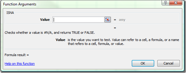
Wed, 03/12/2008 - 10:00am — jethroThe ISNA function is an Information Function. It is is used to return information about the status of a cell, or specifically another functions results. The most common use I have for this function is to validate the VLOOKUP function. If the VLOOKUP function is looking for a value that can not be found in the lookup range, then it will return #N/A as the result. Thus it is good to wrap that function in an IF Statement using the ISNA function to replace the #N/A results with something else – e.g. a text string such as “error” or maybe a zero.
=IF(ISNA(VLOOKUP(A1,$B:$B,1,FALSE))=TRUE,"error",VLOOKUP(A1,$B:$B,1,FALSE))
Remember the ISNA function returns a TRUE or FALSE. These equate to a 1 or 0 so can be used in formulas such as array formulas as well.
Excel Function of the Week - VALUE
Tue, 25/11/2008 - 12:22pm — jethroThis week we are looking at a very simple but a very powerful function.
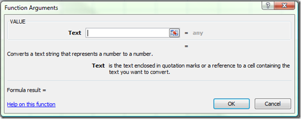
The VALUE function is very easy to use, just type =VALUE(text) in a cell where text is a cell reference is a valid cell address e.g. A1 or T45 or a cell name – e.g. my_cell or just some text. It must represent a number.
The uses of this function are wide. I use it regularly in the following scenarios:
- converting values imported from a CSV file or TEXT file that are actually formatted as text or general. This allows you to use the numbers as actual values and sum them etc. Use =VALUE(A1).
- converting a number string that has been extracted from a text string. E.g. you have a cell A1 with text in it like 1245NAME and you need to get the 1245 out. Use =VALUE(LEFT(A1,4)) to extract the first 4 characters as a text string and then convert it to a number.
- converting a number constructed using CONCATENATE or joins to make. This is very useful for dates. Eg =DAY(TODAY())&"/"&MONTH(TODAY())&"/2020" gies us todays date in the year 2020. However it is not a value, but a text string. Adding VALUE like this =VALUE(DAY(TODAY())&"/"&MONTH(TODAY())&"/2020") turns it into a date serial number. This can then be formatted as a date, and used as a date in calculations.
the Excel help provides this example:
- =VALUE("16:48:00")-VALUE("12:00:00") The serial number equivalent to 4 hours and 48 minutes, which is "16:48:00"-"12:00:00" (0.2 or 4:48)
This Weeks Web Roundup
Thu, 20/11/2008 - 3:32am — jethroTime to unload the browser again. And I have some great stuff for you all this week. Starting with some geek humour as well as some new toys and news.
 Geeks are Sexy post a YouTube video of the Big Bang Theory and Rock, Paper, Scissors, Lizard, Spock, their use of the extended version of Rock, Paper, Scissors. Check it out!
HP has suddenly become an Excel Tips website! These three pages were linked in their last newsletter.
- Go chart crazy with Excel 2007
- Excel tip: make printing easier
- Excel tip: Data entry made easy with AutoFill
Some great news on the Windows Live front.
First of all A note about Hotmail, SkyDrive and Photos storage space from LiveSide advising that there is now a massive 50GB o free space online available to you as follows:


Recent comments
10 years 23 weeks ago
10 years 24 weeks ago
10 years 25 weeks ago
10 years 25 weeks ago
10 years 25 weeks ago
10 years 25 weeks ago
10 years 25 weeks ago
10 years 25 weeks ago
10 years 25 weeks ago
10 years 25 weeks ago