Spy Journal 3.0 Filtering the web for you

Possibly one of the most powerful easy to use formulas in Excel is the SUMIF formula.

It is very easy to use once you get your head around its syntax and it is extremely useful in all sorts of scenarios.

Here is the Microsoft Excel Explanation.

You use the SUMIF function to sum the values in a range (Two or more cells on a sheet. The cells in a range can be adjacent or nonadjacent.) that meet criteria that you specify. For example, suppose that in a column that contains numbers, you want to sum only the values that are larger than 5.

Syntax SUMIF(range, criteria, [sum_range])

I will explain that below more simply.

First let me explain some common scenarios where you might use SUMIF. Hopefully from there you can envisage similar scenarios for your own circumstances.

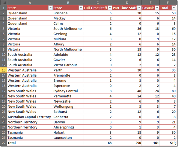
You have a list of names and values – maybe pays or scores or totals of times you beat them in darts matches or numbers of volunteers in each division or county. When the names appear more than once – e.g. you might have several different staff categories in each store across each state as per the example below.

Lets say you want to sum the total number of Part Time Employees in South Australia across all stores.

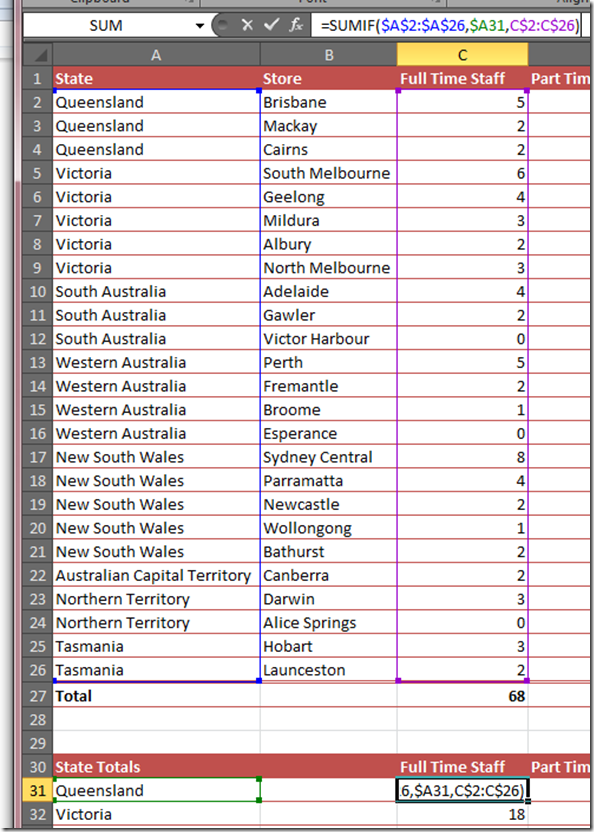
I am going to show you a summary table below this one that provides all the results for each staff category for each State and then explain how this was done using one simple formula. An understanding of ABSOLUTE and RELATIVE references is important.

The formula was created once and then copied to all the State rows and Staff type columns.

It is =SUMIF($A$2:$A$26,$A31,C$2:C$26). I’ll explain each component below the screenshot.

The Syntax for this formula is quite simple once you understand it. I’m going to explain in plain English. Dear Excel. Please look in the list of names and find every name the same as this one (e.g. Queensland). Every time you find one add the value of the Full time Staff for that row. I want to see the total of all of them please. Thank you.

Okay – and now for a little more Excel language.

Look in column A cells 2-31 for every  instance of the value in Cell A31 and sum the value in column C. Total them all up.

And now breaking down the formula itself.

SUMIF (sum when this is true) cells A2:A31 = “Queensland” and the relative value in Column C.

=SUMIF($A$2:$A$26,$A31,C$2:C$26).

I’m using the absolute $ references to lock things up so that this formula can be copied down and across my State summary table.

So $A$2:$A$26 is locked in both directions. no matter where i copy this formula on this sheet it will always look in that range.

$A31 is locking the lookup value (criteria) in the column. So if i copy down it is relative but if i copy across it is fixed.

C$2:C$26 is locked to the rows but relative to the columns. this means it will always look in rows 2-26 but it will change to be the same column as the cell it is copied to.

I trust that helps you – as always comments requesting specific help with this formula will be responded to in the comments. People who ask me to review their work files and email me a file will be charged US$120 an hour.