Spy Journal 3.0 Filtering the web for you

A while ago a reader named Jeremy sent me a request. Sorry I took so long to respond Jeremy – but I’ve finally done this and here are the results.

How can I delete an entire row based on the font color in column A?

I want do delete every row between A2 and A1000 where the font color is black or automatic. I have tried various alterations of the codes below.

Jeremy supplied several procedures, none of which worked correctly.

I have built a very simple version that does what is needed. I know that this is not good code, but it provides a good starting point. And it works. Anybody who needs to use the guts of it (the selection and deletion based on the font colour) can take that and apply it to whatever ranges they need to.

Here is the scenario.

1. You have a range of cells that have been coloured with the automatic font colour. (this could be any colour – you would just need to change the colour index in the code.)
2. You have some items that have been coloured with a different colour.
3. You need to delete the entire row of any cell that has not been coloured specially, ie all the automatic colour cells.

While looking at previous posts to choose a different function for this weeks post I noticed that I have never written a post specifically about the most commonly used function in Excel, the SUM function.

So today’s post remedies that. Note this post is based on Excel 2010. Most of this is still relevant in Excel 2003 and Excel 2007 is largely the same as 2010. The main difference is the ribbon references in Excel 2007/2010 vs the toolbar in 2003.

First the Official Excel Help information.

Description

The SUM function adds all the numbers that you specify as arguments. Each argument can be a range, a cell reference, an array, a constant, a formula, or the result from another function. For example, SUM(A1:A5) adds all the numbers that are contained in cells A1 through A5. For another example, SUM(A1, A3, A5) adds the numbers that are contained in cells A1, A3, and A5.

Syntax

SUM(number1,[number2],...])
The SUM function syntax has the following arguments:
number1    Required. The first number argument that you want to add.
number2,,...    Optional. Number arguments 2 to 255 that you want to add.

Remarks

If an argument is an array or reference, only numbers in that array or reference are counted. Empty cells, logical values, or text in the array or reference are ignored.
If any arguments are error values, or if any arguments are text that cannot be translated into numbers, Excel displays an error.

As the title says this just an introduction. Its aimed at non power users who have recently moved to Office 2010 or 2007 from Excel 2003.

The main reason for this article is to demonstrate the basic use of the new table features and the ribbon features available to users.

I am going to start with showing you how to make a table from existing data and demonstrate a few of the ribbon features. I wont be going into anything too complicated in this post. Depending on feedback I might write some more specific detailed feature articles on table components and using tables later including converting tables back to ranges..

So how do we make a table – its actually very simple. In the following screenshots you will see a fairly typical spreadsheet with some information in it. I will show you how to turn that into a table.

Select any cell in the table.

From the Home Tab on the Ribbon click on the Format as Table Button.

Possibly one of the most powerful easy to use formulas in Excel is the SUMIF formula.

It is very easy to use once you get your head around its syntax and it is extremely useful in all sorts of scenarios.

Here is the Microsoft Excel Explanation.

You use the SUMIF function to sum the values in a range (Two or more cells on a sheet. The cells in a range can be adjacent or nonadjacent.) that meet criteria that you specify. For example, suppose that in a column that contains numbers, you want to sum only the values that are larger than 5.

Syntax SUMIF(range, criteria, [sum_range])

I will explain that below more simply.

First let me explain some common scenarios where you might use SUMIF. Hopefully from there you can envisage similar scenarios for your own circumstances.

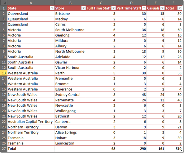
You have a list of names and values – maybe pays or scores or totals of times you beat them in darts matches or numbers of volunteers in each division or county. When the names appear more than once – e.g. you might have several different staff categories in each store across each state as per the example below.

Lets say you want to sum the total number of Part Time Employees in South Australia across all stores.

I am going to show you a summary table below this one that provides all the results for each staff category for each State and then explain how this was done using one simple formula. An understanding of ABSOLUTE and RELATIVE references is important.